
Efficient Large-scale Road Inspection Routing
Yujie Chen
1
, Peter Cowling
1
, Stephen Remde
2
and Fiona Polack
1
1
YCCSA, Computer Science Department, University of York, York, U.K.
2
Gaist Solutions Limited, Lancaster, U.K.
Keywords:
Graph reduction, Routing, Chinese Postman Problem.
Abstract:
Gaist Solutions Ltd. carries out large scale surveys for UK road inspection. To estimate the total distance that
vehicles travel, we model routing as a Chinese Postman Problem. We propose a novel graph reduction ap-
proach that dramatically speeds up the calculation of the Chinese Postman Tour for large-scale road networks.
Because the analysis of large road-network graphs is now possible, planners can explore the effects of changes
to traditional inspection techniques and scheduling. Case studies of road networks from six UK cities and the
county of Norfolk are tested. The graph reduction process is also analysed on ten randomly generated road
networks with different characteristics, to show its ability and give advice for suitable use.
1 INTRODUCTION
In the UK, local governments maintain roads for pub-
lic utility and safety. We can model route inspection
as a Chinese Postman Problem (CPP). To estimate the
total distance that vehicles travel to inspect all routes,
a very large-scale CPP must be solved. Published ap-
proaches to deriving a Chinese Postman Tour (CPT)
are computationally demanding and do not scale to
large graphs. Graphs that represent road networks
are characterised by vertices with low degree (e.g.
T junctions of degree 3 or crossroads of degree 4).
Also, roads in residential areas have a strong branched
structure. By understanding these characteristics, we
propose a graph reduction approach to improve the
efficiency of routing large-scale real-world road in-
spection problem. Our road-inspection routes are for
seven large-scale road networks monitored by Gaist
Solutions Ltd. in partnership with the UK local coun-
cils of Blackpool, Southend, Manchester, Stockport,
Halton, Warrington, and the rural county of Norfolk
(road lengths of 515, 508, 1,315, 945, 619, 879 and
26,243 kilometres, respectively). We also evaluate
our graph reduction approach using simulated net-
works.
Section 2 introduces road networks and their
transformation to abstract graphs. Section 3 outlines
CPP solutions and their scalability limitations. The
graph reduction process is introduced in Section 4,
then the application of the conventional CPT solution
and of two variations using heuristics are introduced
in Section 5. Section 6 and 7 compare our results over
seven local authority road networks and ten simulated
data sets. Conclusions are presented in Section 8.
2 REAL-WORLD ROAD
NETWORKS
UK local authority road networks are designated as
1-lane, 2-lane, 3-lane and 4-lane single carriageways
or 2-lane dual carriageways (with a central reserva-
tion). We represent a road network as an undirected
graph G(V,E). Vertices V represent the data collec-
tion points: some are junctions or dead ends, but oth-
ers are simply bends in the road. Edges E represent
the roads that link vertices.
In our inspection problems, up to 3 lanes can be
monitored in one pass. Figure 1 shows 1-lane, 2-lane
and 3-lane single carriageways represented by a sin-
gle undirected edge. Figure 2 shows 4-lane single car-
riageways and dual carriageways represented as two,
parallel undirected edges. A close road is represented
as a loop (Figure 3), and a cul-de-sac is represented
as an degree-1 vertex (Figure 4).
The road information was originally collected
street by street, but has some errors or omissions. Be-
fore creating the graph representation, we pre-process
and label intersections as vertices, as follows.
• All degree-2 vertices are removed, since they do
not represent intersections, and thus have no im-
304
Chen, Y., Cowling, P., Remde, S. and Polack, F.
Efficient Large-scale Road Inspection Routing.
DOI: 10.5220/0005749203040312
In Proceedings of 5th the International Conference on Operations Research and Enterprise Systems (ICORES 2016), pages 304-312
ISBN: 978-989-758-171-7
Copyright
c
2016 by SCITEPRESS – Science and Technology Publications, Lda. All rights reserved

(a) 1-lane single carriageway (b) 2-lane single carriageway
(c) 3-lane single carriageway (d) Graph representation
Figure 1: Graph representation of single carriageway roads.
(a) 4-lane single carriage-
way
(b) 2-lane dual carriageway
(c) Graph representation
Figure 2: Graph representation of 4-lane single carriageway
and 2-lane dual carriageway.
pact on the construction or distance of inspection
tours. For all degree-2 vertices, v
k
, e(v
i
,v
k
) and
e(v
k
,v
j
) are replaced by a single edge, e(v
i
,v
j
),
with length l((v
i
,v
j
)) = l((v
i
,v
k
)) + l((v
k
,v
j
)).
• We assume that an intersection has been omitted
if the data indicates that a road terminates close
to another road or road-termination point. The
critical value for “close”, is set at ε = 3 me-
tres, based on our analysis of the original data.
So, where the distance from a degree-1 vertex
v
k
to an edge e(v
i
,v
j
) is less than ε, the edge
e(v
i
,v
j
) is replaced by two new edges e(v
i
,v
k
)
and e(v
k
,v
j
). Or, where the distance between two
degree-1 vertices is smaller than some ε, the ver-
tices are merged.
Removal of degree-2 vertices significantly reduces
the size of the graphs, as shown in Table 1.
3 CPP AND THE CHALLENGE
OF SCALE
CPP was formulated by a Chinese mathematician: A
mailman has to deliver mail to every road of his ser-
vice area before returning to the post office. The prob-
lem is to find the shortest walking distance for the
mailman. (Guan (1962)).
3.1 Edmonds’ Approach
To solve a standard CPP, a CPT is derived by adding
the smallest possible number of edges to construct
(a) Close (b) Graph representation
Figure 3: Graph representation of close roads.
(a) Bulb (b)Dead-end (c)Representation
Figure 4: Graph representation of cul-de-sacs.
an Eulerian graph, which must then contain an Euler
tour. Edmonds and Johnson (1973) provide a widely-
used CPP approach that is polynomial on the number
of vertices and edges, (and does not scale well to large
graphs) as follows.
Step 1: From an undirected graph G(V, E), find the
shortest path between all pairs of odd-degree vertices.
Two algorithms are commonly used in this
step. The most efficient implementations
of Dijkstra’s algorithm (Dijkstra (1959)),
a single-source shortest-path algorithm, can
achieve O(m + n logn), where m is the num-
ber of edges (Fredman and Tarjan (1987)).
Floyd (1962) and others developed an algo-
rithm, now known as the Floyd-Warshall al-
gorithm (FW), of complexity O(n
3
) where n
is the number of vertices.
Tested on our large-scale sparse graphs, FW system-
atically outperforms Dijkstra’s algorithm. However,
the computational efficiency of FW can itself be sig-
nificantly improved by reducing the number of nodes
in a graph, e.g. by applying graph reduction.
Step 2: Find the minimum-cost perfect matching,
M, of odd-degree vertices.
The best-known minimum-cost per-
fect matching implementation (Gabow
(1990)), using the blossom algorithm (Ed-
monds (1965); Edmonds and Johnson
(1973)), is also computationally expensive
(O(n(m + nlogn))). Kolmogorov (2009) has
an implementation which achieves O(n
2
m).
Again, the complexity of the algorithm is dependent
on the number of edges and vertices in the graph.
Efficient Large-scale Road Inspection Routing
305

Table 1: Number of vertices before and after removal of 2-degree vertices for seven UK local authority road networks.
Vertices Blackpool Southend Manchester Stockport Halton Warrington Norfolk
Total 26302 22864 45408 44470 29610 24518 549345
less degree-2s 5103 4571 13337 8665 4796 7471 44912
Step 3: Add extra edges to connect all matched
pairs of vertices through the shortest path in G, to cre-
ate an Eulerian graph.
Step 4: Find the CPT: an Euler tour in the Eulerian
graph. Then, the length, l
CPT
, of the identified Chi-
nese Postman Tour (CPT) is:
l
CPT
=
∑
e∈E
l(e) + l(M)
The best known approach to finding an Euler
tour is Hierholzer’s algorithm (Hierholzer and
Wiener (1873)), with time complexity O(m).
Another widely applied approach, by Fleury
(1883), achieves O(m
2
).
3.2 Other Approaches
Apart from Edmonds’ CPP solution, Laporte (1997)
introduces methods of transforming an arc routing
problem into an equivalent TSP. This approach is also
used by Irnich (2008) to solve a large-scale real-world
postman problem. Heuristics for the TSP can then be
used to solve the transformed CPP. For an extensive
bibliography of CPP variations and solvers, see (Cor-
ber
´
an and Laporte (2015)).
3.3 Road Inspection and the CPP Model
An advanced inspection vehicle is able to monitor up
to three lanes of a typical UK road in one traversal.
Hence, to achieve the road inspection task, each edge
in the abstract graph has to be visited at least once.
The total travel distance is the length of Chinese Post-
man Tour (CPT) (Guan (1962); Thimbleby (2003)).
Representing a road network as an undirected
graph ignores the necessarily directed nature of 4-
lane single carriageways and dual carriageways (Fig-
ure 2). However, we generate an Eulerian graph from
a given road network, so according to Lemma 3.1 we
can always find a CPT that passes complementary di-
rections of parallel edges, and is thus legal for 4-lane
single and dual carriageways.
Lemma 3.1. If a graph G(V,E) is eulerian and edge
{v, w} appears twice in E, then there is an Euler tour
of G where {v,w} is travelled in both directions {v, w}
and {w, v}.
Proof. Suppose that there is an Euler tour v−w−x
1
−
x
1
−...−x
n
−v−w−y
1
−y
2
−...−y
n
−v, where edge
(v, w) is travelled in the same direction both times.
Then v − w − v − y
n
− y
n−1
− ... − y
1
− w − x
1
− x
2
−
...x
n
−v is another Euler tour where edge (v,w) is trav-
elled in both directions.
4 REDUCTION OF LARGE
GRAPHS
As noted above, the greatest contribution to compu-
tational complexity of the algorithms used to derive
a CPT is the number of vertices and edges. Our
graph reduction applies graph contraction techniques
as used in graph minor theory (Chartrand and Oeller-
mann (1993); Lov
´
asz (2006)). Edge contraction is a
fundamental operation in graph minors which deletes
an edge from a graph G and merges the two end
points. Here, we propose a novel graph reduction
method to decrease the size of the calculations whilst
maintaining the necessary characteristics of the origi-
nal graph to reconstruct a CPT. After the data prepara-
tion described in Section 2, each road network is rep-
resented as a finite undirected graph which contains
parallel edges and self-loops. All degree-2 vertices
have been removed.
4.1 Reduction Process
Let V
even
and V
odd
describe the even-degree vertex set
and odd-degree vertex set, respectively, of our graph
G(V,E). l(v
i
,v
j
) represents the length of the shortest
edge between vertices v
i
and v
j
. If there is no direct
connection between v
i
and v
j
, l(v
i
,v
j
) = ∞. For all
vertices v
i
, l(v
i
,v
i
) = 0. The shortest path between v
i
and v
j
in the graph G is represented as p(v
i
,v
j
).
We delete vertices systematically, but record the
length and location of removed edges incident to
degree-1 vertices in a structure, E
∗
. Figure 5 shows
how this works on a stylised representation of a road
network graph. We make the following observations.
1. Deleting a self-loop from a graph does not change
the parity of a vertex’s degree.
2. The shortest path p(v
i
,v
j
) between vertex v
i
and
vertex v
j
does not include any self-loops.
3. The paths P of the minimum cost matching
M(V
odd
) include all the edges connected to
ICORES 2016 - 5th International Conference on Operations Research and Enterprise Systems
306

Figure 5: Systematic reduction of an undirected graph. (a) is the graph after removal or degree-2 vertices, with the matching
M
odd
shown in dashed lines. (b) shows the graph after removal of degree-1 vertices, with their originally connected edges
recorded in E
∗
. (c)-(g) show the result of repeating these steps – here, the result is a null graph. White nodes have degree 1;
striped nodes have even degree and black nodes have odd degree.
degree-1 vertices: if you reach a dead end, then
you have to leave the way you entered.
4. If a shortest path between vertex v
i
and v
j
is
p(v
i
,v
j
) = (v
i
,v
i+1
,v
i+2
,...,v
j
), then the short-
est path between v
i+1
and v
j
is p(v
i+1
,v
j
) =
(v
i+1
,v
i+2
,...,v
j
).
5. When deleting a degree-1 vertex and its adjacent
edge, the total number of odd degree vertices is
either unchanged or reduced by 2.
From these observations, we deduce:
1: Deleting a self-loop (v
i
,v
i
) from a graph G will
not change the paths in the minimum perfect
matching M(V
odd
) of an undirected graph.
2: There is a path set P of the matching M(V
odd
)
of the original graph G (dashed lines in Figure
5(a)) that equals the deleted edges E
∗
incident
to degree-1 vertices (as shown by the E
∗
in Fig-
ure 5(b)), plus a path set P
0
in the new matching
M
0
(V
odd
) of the simplified graph G
0
(dashed lines
in Figure 5(b)), such that, P = E
∗
∪ P
0
.
4.2 Further Reduction to Remove
Even-degree Vertices
The graph reduction results in a simplified graph G
0
,
plus a record of all deleted edges that were inci-
dent to degree-1 vertices, E
∗
in the reduction process.
We observe that the FW algorithm used to find the
least distance between pairs of odd-degree vertices
has complexity exponential in the number of vertices,
and graph G
0
still contains many even-degree vertices
which do not affect the shortest path calculation. Thus
we further reduce the graph by deleting these even-
degree vertices.
Our preferred approach to even-degree vertex
deletion detects and deletes all even-degree vertices in
G
0
without affecting the shortest connection and dis-
tance between other vertices. Deleting vertices with
degree higher than three may increase the total num-
ber of edges, but always reduces the total number
of vertices. The complexity of deleting each even-
degree vertex v
i
∈ V
even
is ((m(v
i
)(m(v
i
) − 1)) / 2),
where m(v
i
) is the number of edges incident to vertex
v
i
.
5 CPT DERIVATION
Having achieved a reduced graph, we apply Ed-
monds’ conventional CPT derivation (see Section
3.1), and also two alternative approaches that replace
resource-intensive algorithms with heuristics.
5.1 Applying Edmonds’ CPT Derivation
Our graph reduction approach makes it computation-
ally feasible to use the conventional CPT derivation
algorithms (see Section 3.1) on large networks. Be-
cause the graph reduction reduces the number of ver-
tices considered, its effects are principally in step 1,
the use of FW to derive the shortest path between all
pairs of odd-degree vertices.
In step 2, we use the blossom algorithm to find the
minimum-cost perfect matching, M(V
0
odd
) of graph
Efficient Large-scale Road Inspection Routing
307

Table 2: Labelling of the combinations of the three graph forms and three solvers applied, used in subsequent figures and
tables. For details see text. FW = Floyd-Warshall Algorighm (step 1). Blossom, greedy and BFS are used for matching (step
2). GR = Graph reconstruction (step 3). HA = Hierholzer Algorithm to find the CPT (step 4).
Steps 1-4
Graph FW, blossom, GR, HA FW, Greedy, GR, HA BFS, GR, HA
graph with 2-degree vertices
removed
m1 m2 m3
... and reduction applied m4 m5 m6
... and all even degree ver-
tices removed
m7 m8 m9
G
0
. The length of the minimum perfect matchings is
represented as l
M(V
0
odd
)
. The length l
CPT
of the CPT of
the original graph G is:
l
CPT
=
∑
e∈E
l(e) +
∑
e∈E
∗
l(e) + l
M(V
0
odd
)
(1)
To construct an Eulerian graph from the original
graph G (step 3), using Deduction 2, we only need to
re-insert the edges recorded in E
∗
and M(V
0
odd
) to the
original graph G. Thence, we use Hierholzer’s algo-
rithm to find the Euler tour (step 4). To generate a
CPT in a real world situation, when Hierholzer’s al-
gorithm meets a vertex connected to 4-lane single car-
riageway or dual carriageway edges, priority is given
to the edge whose underlying direction is away from
this vertex.
5.2 Heuristic Alternatives for CPT
We explore potential improvements in computational
efficiency of CPT derivation for our large, sparse
graphs, by introducing simple heuristic alternatives to
the blossom algorithm for minimum-cost matching in
step 2, above.
Greedy method (greedy) is a heuristic approach
to constructing a matching where shortest distances
between pairs of vertices are known. The greedy al-
gorithm 1, which is run after FW, is based on those by
(Kurtzberg (1962)) and (Reingold and Tarjan (1981)).
Algorithm 1: Greedy heuristic for matching.
V L is a list of all the vertices, v
i
in a given graph
while V L contains at least two vertices do
Choose the pair of vertices with shortest distance
(v
i
,v
j
) ∈ V L
Add (v
i
,v
j
) to the matching M
delete v
i
,v
j
from V L
end while
Return M
Breadth first search (BFS) is a basic search:
each unmatched odd-degree vertex v
i
in graph G be-
comes the root of a BFS to find the next unmatched
odd-degree vertex v
j
. The two vertices v
j
and v
i
are
a matching pair and the path from v
i
to v
j
in the BFS
tree is the matching path. The BFS terminates when
there are no unmatched odd-degree vertices left. BFS
does not need to run FW first, which should signif-
icantly improve the computational efficiency of the
CPT derivation.
6 RESULTS ON REAL-WORLD
DATA
Our experiments run each of the variant CPT deriva-
tions on three versions of each road network graph:
with removal of degree-2 vertices (Section 2), then
also with graph reduction (Section 4.1), and finally
also with removal of all even-degree vertices (Sec-
tion 4.2). Table 2 introduces labels m1...m9 for these
combinations. The experiments compare the compu-
tation time for each combination, on a standard desk-
top PC: Intel i7-3770 CPU at 3.40 GHz with 24GB
memory under the Windows 7 operation system.
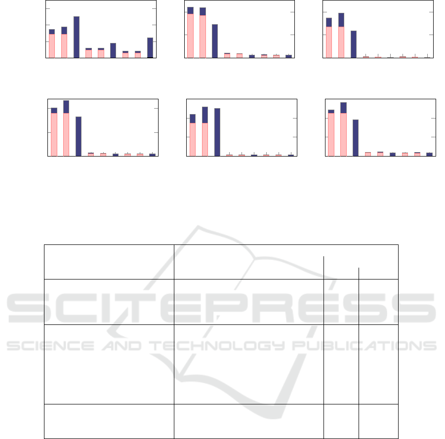
Figure 6 plots the CPU time taken for each experi-
ment. For each road network, the graph reduction and
graph reconstruction times are negligible, and do not
show up on this scale. In all network cases, the graph
reduction (m4 – m9) shows significantly lower over-
all CPU time. The major contributions come from the
time saving in the process of finding the shortest path
(using FW) and the minimum cost matching. This
result demonstrates the importance of our graph re-
duction approach for sparse graphs of this scale.
The results show that, having achieved computa-
tional feasibility through graph reductions, the exact
method, using the blossom algorithm for matching,
outperforms the heuristic approaches. This result is
useful since the blossom approach guarantees to find
the optimal CPT, whereas the heuristic approaches
typically find a close but suboptimal solution.
Table 3 gives numerical results for m1, m4 and
m7 (the blossom-based solvers) on the three versions
of the graphs. The results again emphasise the ef-
ICORES 2016 - 5th International Conference on Operations Research and Enterprise Systems
308

Table 3: CPU time taken to calculate a CPT for each road network using the blossom algorithm matching. The lower right
panel gives total CPU time for each road network and each experiment. Column n is the number of vertices (cf. Table 1);
m the number of edges in the graphs after data cleaning. RT is CPU time for graph reduction. FW is CPU time for the FW
algorithm. MT is CPU time for the blossom algorithm. CT is CPU time to construct the final graph. CPT is CPU time to
extract the final inspection route using the Hierholzer algorithm.
Blackpool (B) Southend (SO)
n m
CPU (s)
n m
CPU (s)
RT FW MT CT
CPT
RT FW MT CT CPT
m1 5103 7124 0 143.32 28.97 0.016
0.187
4571 5738 0 189.84 31.14 0.001 0.202
m4 3398 5419 0.14 45.54 11.11 0.016
0.234
2016 3162 0.14 16.05 4.26 0.001 0.203
m7 2772 10803 0.51 28.84 10.34 0.016
0.016
1746 5922 0.28 10.51 4.25 0.001 0.202
Halton (H) Stockport (ST)
n m
CPU (s)
n m
CPU (s)
RT FW MT CT
CPT
RT FW MT CT CPT
m1 4796 5430 0 134.38 39.44 0.002
0.187
8665 10482 0 910.62 114.21 0.000 0.671
m4 1211 1852 0.15 2.96 1.97 0.001
0.218
3277 5063 0.45 55.91 12.46 0.006 0.826
m7 1148 1970 0.16 2.53 1.96 0.002
0.218
3004 5662 0.53 40.86 11.79 0.003 0.858
Warrington (W) Manchester (M)
n m
CPU (s) CPU (s)
RT FW MT CT
CPT
n m RT FW MT CT CPT
m1 7471 8556 0 343.18 95.32 0.001
0.499
13337 16500 0 4438.04 355.83 0.013 1.58
m4 2136 3218 0.29 10.31 5.84 0.000
0.561
5842 8949 1.02 369.71 47.75 0.015 1.79
m7 2108 3265 0.31 9.78 5.83 0.001
0.561
5486 9622 1.12 306.29 46.71 0.015 1.67
Norfolk (N) Summary
n m
CPU (s) Total CPU(s)
RT FW MT CT
CPT
B SO H ST W M N
m1 44912 53482 0 - - -
-
172 221 174 1025 439 4795 -
m4 15647 23904 18.27 4977.19 5499.49 0.171
34.523
57 21 5 70 17 420 10530
m7 14796 26487 19.66 4227.01 4759.01 0.182
34.881
49 15 5 54 16 356 9041
Table 4: CPT length of seven road networks.
Blackpool Southend Halton
l(CPT) 671.60km 676.02km 917.16km
Stockport Warrington Manchster
l(CPT) 1369.60km 1300.92km 1839.09km
Norfolk
l(CPT) 18268.84km
fect of graph reduction in reducing CPU time. These
methods calculate the optimal CPT of the original
graph, and the distance that vehicles should travel for
road inspection. The CPT length for each network is
shown in Table 4.
7 SIMULATED DATA
EXPERIMENTS
To explore the effect of graph reduction further, we
conducted a set of experiments on randomly gener-
ated graphs, using the blossom-based solvers (as in
m1, m4 and m7).
The random graphs are generated, using an al-
gorithm proposed by Blitzstein and Diaconis (2011),
with a fixed number (1000) of vertices, and with spe-
cific vertex-degree distributions. As shown in Table 5,
we also record average vertex degree of the generated
graphs before and after the initial removal of degree-2
vertices. Three parameter settings of random graphs
(g1, g2, g3) are generated with similar vertex-degree
distribution to the graphs representing the real-world
road networks before any data processing. A further
five parameter settings of random graphs (g4 – g8)
have similar vertex-degree distribution to the graphs
of real-world road networks after removal of degree-2
vertices. There are also two parameter settings of ran-
dom graphs that are dominated by degree-4 (g9) and
degree-5 (g10) vertices. In the random generation, all
edge lengths are set to one.
For each graph, we run the blossom-based solvers
with progressively greater reductions (as for m1, m4
and m7, above). For each experiment, we report the
average of 30 runs, a number selected to give accept-
able total run time but a suitably-low statistical error.
Table 6 presents details of the CPU time taken for
the overall CPT identification process, and then for
the three levels of graph reduction, on each graph.
Each graph reduction makes a big contribution to
the CPU time reduction. The results for the first group
of graphs, those generated to match the vertex de-
gree distribution of the complete road network graphs,
Efficient Large-scale Road Inspection Routing
309
m1
m2
m3
m4
m5
m6
m7
m8
m9
0
100
200
300
Blackpool
Time (s)
m1
m2
m3
m4
m5
m6
m7
m8
m9
0
100
200
Southend
m1
m2
m3
m4
m5
m6
m7
m8
m9
0
100
200
Halton
m1
m2
m3
m4
m5
m6
m7
m8
m9
0
500
1,000
Stockport
Time (s)
m1
m2
m3
m4
m5
m6
m7
m8
m9
0
200
400
600
Warrington
m1
m2
m3
m4
m5
m6
m7
m8
m9
0
2,000
4,000
6,000
Manchster
Figure 6: CPU time for the six road networks. m1 to m3 solve the CPP on graphs with 2-degree vertices removed, which is
the standard approach widely used for network representation. m4 to m6 solve the CPP on graphs after our graph reduction
process, and m7 to m9 solve the CPP on further reduced graphs with all even degree vertices removed. See table 2 definitions.
Table 5: Vertex degree distributions for generated graphs. All generated graphs have 1000 vertices and edges of length 1 only.
parameters
vertex degree average degree
Graph structures 1 2 3 4 5 initial no d-2
degree distribution match:
g1 15% 70% 12% 3% - 2.03 2.1
g2 10% 70% 15% 5% - 2.15 2.5
g3 5% 80% 10% 5% - 2.15 2.75
degree distribution with no
degree-2 vertices:
g4 35% - 60% 5% - 2.35 2.35
g5 35% - 50% 15% - 2.45 2.45
g6 35% - 40% 25% - 2.55 2.55
g7 35% - 40% 10% 15% 2.7 2.7
g8 35% - 40% 5% 20% 2.75 2.75
dominated by high-degree :
g9 20% - 15% 60% 5% 3.3 3.3
g10 20% - 15% 5% 60% 3.85 3.85
show the importance of removing degree-2 vertices.
A further large time saving occurs when the graph re-
duction process (Section 4) is applied. Comparing the
improvement in CPU times between the full graph
reduction (last column of Table 6) and only remov-
ing degree-2 vertices (middle column total), the first
group of graphs show CPU time savings of 95.5%,
90.3% and 78.5%, respectively.
The graphs in group g4 – g8 (and g9, g10) are gen-
erated without degree-2 vertices. For these graphs,
the graph reduction steps also show a very large CPU
time reduction.
For the graphs dominated by higher-degree ver-
tices, g9 and g10, the results again show that graph
reduction leads to time reductions. However, for g9
which is dominated by degree-4 vertices (60% of all
vertices), the further reduction step, to remove all
even vertices, is by far the most computationally ex-
pensive step (three times the CPU time for just remov-
ing degree-one vertices), making the reduction more
expensive than solving the unreduced graph. In this
case, the last column of Table 6 shows that there is a
very large CPU time overhead for deleting the signifi-
cant number of degree-4 vertices and any other higher
even-degree vertices. Hence, only applying the reduc-
tion process in section 4.1, is the most efficient ap-
proach in this situation. In contrast, the graphs domi-
nated by degree-five vertices, g10, show a pattern that
is consistent with the graphs that are generated to have
similar degree to the real road network graphs.
ICORES 2016 - 5th International Conference on Operations Research and Enterprise Systems
310

Table 6: CPU time for CPT tour extraction on generated random graphs g1 – g10, showing the effect of graph reductions.
Lowest overall CPU times for each graph type are in emboldened.
CPU(ms)
Graph FW, blossom removing and reduction and removing
structure GR, HA degree 2 applied all even degree
reduction total reduction total reduction total
g1 19691.82 10.66 577.56 11.61 29.49 12.07 25.91
g2 19616.67 10.21 568.72 11.36 86.71 12.93 54.86
g3 19522.89 11.30 183.39 11.75 60.01 15.18 39.37
g4 20464.62 - - 6.34 1831.37 7.76 1436.3
g5 20312.60 - - 6.22 2086.82 14.64 1062.11
g6 20582.34 - - 5.55 2528.90 863.95 1666.97
g7 20433.91 - - 4.88 2780.43 13.07 1414.97
g8 20359.70 - - 4.87 2810.04 10.99 1622.76
g9 20339.90 - - 3.88 8468.91 248918.2 249369.4
g10 20407.10 - - 3.68 9209.61 17.08 4992.87
8 CONCLUSIONS
To estimate the total distance that vehicles need to
travel for road inspection tasks, we model this prob-
lem as a CPP. We present a systematic method for pro-
cessing raw data from road surveys, applicable road
networks in general, and show further abstract graph
representations. We propose a graph reduction tech-
nique that dramatically speeds up the calculation of
CPT of very large-scale road networks.
Our graph reduction technique is notably helpful
on sparse graph like real-world road networks; even
the graph of a UK county road network is amenable
to CPT route calculation on a standard PC. For road
networks in residential areas, the reduction helps to
manage the many branch roads, close road and cul-
de-sacs which lead to complex graph structures.
Our approach is applicable to any road-tour
derivation, such as large-scale door-to-door delivery
or monitoring services and rubbish collection; the ef-
ficient computational approach can facilitate experi-
mentation with innovative policies and techniques for
route planning.
ACKNOWLEDGEMENTS
The authors would like to thank Gaist Solutions Ltd.
for providing data and domain knowledge. This re-
search is part of the LSCITS project funded by the
Engineering and physical sciences research council
(EPSRC).
REFERENCES
Blitzstein, J. and Diaconis, P. (2011). A sequential im-
portance sampling algorithm for generating random
graphs with prescribed degrees. Internet Mathemat-
ics, 6(4):489–522.
Chartrand, G. and Oellermann, O. (1993). Graph Minors. In
Applied and Algorithmic Graph Theory, pages 277–
281. McGraw-Hill.
Corber
´
an,
´
A. and Laporte, G. (2015). Arc routing: prob-
lems, methods, and applications. SIAM.
Dijkstra, E. W. (1959). A note on two problems in connex-
ion with graphs. Numerische mathematik, 1(1):269–
271.
Edmonds, J. (1965). Paths, trees, and flowers. Canadian
Journal of mathematics, 17(3):449–467.
Edmonds, J. and Johnson, E. L. (1973). Matching, Euler
tours and the Chinese postman. Mathematical pro-
gramming, 5(1):88–124.
Fleury, M. (1883). Deux problemes de geometrie de
situation. Journal de mathematiques elementaires,
2(2):257–261.
Floyd, R. W. (1962). Algorithm 97: Shortest Path. Commu-
nications of the ACM, 5(6):345.
Fredman, M. L. and Tarjan, R. E. (1987). Fibonacci heaps
and their uses in improved network optimization algo-
rithms. Journal of the ACM, 34(3):596–615.
Gabow, H. N. (1990). Data structures for weighted match-
ing and nearest common ancestors with linking. In
Proceedings of the First Annual ACM-SIAM Sympo-
sium on Discrete Algorithms, pages 434–443. Society
for Industrial and Applied Mathematics.
Guan, M. (1962). Graphic programming using odd or even
points. Chinese Math, 1(273-277):110.
Hierholzer, C. and Wiener, C. (1873). Ueber die
M
¨
oglichkeit, einen Linienzug ohne Wiederholung und
ohne Unterbrechung zu umfahren. Mathematische An-
nalen, 6(1):30–32.
Efficient Large-scale Road Inspection Routing
311

Irnich, S. (2008). Solution of real-world postman prob-
lems. European Journal of Operational Research,
190(1):52–67.
Kolmogorov, V. (2009). Blossom V: a new implementation
of a minimum cost perfect matching algorithm. Math-
ematical Programming Computation, 1(1):43–67.
Kurtzberg, J. M. (1962). On approximation methods for
the assignment problem. Journal of the ACM (JACM),
9(4):419–439.
Laporte, G. (1997). Modeling and solving several
classes of arc routing problems as traveling sales-
man problems. Computers & operations research,
24(11):1057–1061.
Lov
´
asz, L. (2006). Graph minor theory. Bulletin of the
American Mathematical Society, 43(1):75–86.
Reingold, E. M. and Tarjan, R. E. (1981). On a greedy
heuristic for complete matching. SIAM Journal on
Computing, 10(4):676–681.
Thimbleby, H. (2003). The directed Chinese Postman Prob-
lem. Software Practice and Experience, 33(11):1081–
1096.
ICORES 2016 - 5th International Conference on Operations Research and Enterprise Systems
312
