Investigation on Compressed Wavefront Sensing in Freeform Surface

Measurements

Eddy Chow Mun Tik

, Xin Wang

, Ningqun Guo

, Ching SeongTan

and Kuew Wai Chew

School of Engineering, Monash University Malaysia, Jalan Lagoon Selatan, Bandar Sunway, Subang Jaya, Malaysia

Faculty of Engineering, Multimedia University, Cyberjaya, Malaysia

Faculty of Engineering and Science, University Tunku Abdul Rahman, Kampar, Malasyia

Shack-Hartmann Wavefront Sensing, Compressed Sensing, Freeform Surface Measurement.

Abstract: In this paper, conventional modal wavefront reconstruction is compared with compressed wavefront sensing

to reconstruct freeform surface profiles using the Shack-Hartmann wavefront sensor. The modal wavefront

reconstruction represents the phase or the wavefront in the Zernike domain. The compressed wavefront

sensing method based on the sparse Zernike representation (SPARZER) represents the phase slopes in the

Zernike domain. The effectiveness of compressed wavefront sensing in freeform surface profile

measurements is investigated.

1 INTRODUCTION

The Shack-Hartmann wavefront sensor has been

popular due to its simplicity in measuring the shape

of a wavefront. Since the start of its development in

the late 1960s for the use of improving images

captured from ground telescopes (Platt & Shack,

2001), its applications expanded to measurement of

aberrations of the eye and optical component

characterization among others (Schwiegerling &

Neal, 2005). There have been a great amount of

research to improve the accuracy of the Shack-

Hartmann wavefront sensor. This includes new

centroid detection algorithms (Yin, et al., 2009), de-

noising centroid images (Basden, et al., 2015), use of

new basis functions (Lundstrom & Unsbo, 2004), and

new wavefront reconstruction algorithms (Rostami,

et al., 2012).

Compressive sensing meanwhile is a great

optimization technique to recover sparse signals even

when the sampling rate is lower than required by the

Shannon-Nyquist sampling theorem (Donoho, 2006).

This is done by solving underdetermined linear

systems where the signal is sparse in a particular

domain. Another requirement is the incoherence

between the sampling and the representing domains

e.g. the time and frequency domains (Candes &

Romberg, 2005). The linear equations are solved

using l1 minimization, which does not have an

analytical solution. It is solved using iterative

numerical methods such as linear programming etc.

(Candes, et al., 2006)

Application of compressed sensing on the Shack-

Hartmann wavefront sensor is possible because there

exist a sparse representation of the projected

wavefront. A popular representation of the wavefront

is in the Zernike domain (Noll, 1976). Early work has

shown different implementations of compressive

sensing in Shack-Hartmann wavefront sensors. This

includes the representation of phase slopes in the

Zernike domain (Polans, et al., 2014), and defining

the sensing domain as the Dirac comb (Hosseini &

Michailovich, 2009).

The use of Shack-Hartmann wavefront sensing on

free-form surfaces presents some challenges due to

the nature of freeform surfaces themselves. Due to

large slopes or curvature of freeform surfaces, the

focal spot on the image sensor could be distorted

(Guo, et al., 2013). This causes the centroid detection

algorithm to be inaccurate, and thus producing

inaccurate phase slope measurements. Compressive

wavefront sensing has shown to reconstruct

wavefronts accurately even with noisy measurements

(Polans, et al., 2014).

154

Tik, E., Wang, X., Guo, N., SeongTan, C. and Chew, K.

Investigation on Compressed Wavefront Sensing in Freeform Surface Measurements.

DOI: 10.5220/0005743901520157

In Proceedings of the 4th International Conference on Photonics, Optics and Laser Technology (PHOTOPTICS 2016), pages 154-159

ISBN: 978-989-758-174-8

2 THEORY

2.1 Modal Wavefront Reconstruction

The classic modal reconstruction of Shack-Hartmann

wavefront sensors uses the least squares optimization

to solve the linear equations which approximate the

wavefront to a summation of some decomposed

polynomials (Dai, 1994).

=











(1)

Where a

is the ith coefficient, and Z

is the ith

polynomial. The commonly used polynomials are the

Zernike polynomials and Fourier transforms.

The information obtained from the Shack-

Hartmann wavefront sensor meanwhile are the phase

slopes in the x and y direction of phase Φ, which can

be approximated to the distance of a focal spot to its

reference divided by the focal length of the lenslets.





=

∆





(2)





∆



=





(3)

For a Shack-Hartmann wavefront sensor with

lenslets of n×n grid, the number of phase slope

measurements will be 2n

. In matrix form, the above

equations can be represented as

=

(4)

Where F is the column matrix of phase slope

measurements, E is matrix of the partial differentials

of polynomials Z in the x and y direction, and A is the

matrix of coefficients of Z.

The elements in matrix E, are the average Zernike

derivatives over the corresponding sub-apertures of

the Shack-Hartmann wavefront sensor.

The least squares solution to the above equation

would be



=(



)









(5)

2.2 Compressed Wavefront Sensing

The method used for compressed wavefront sensing

is the sparse Zernike representation (SPARZER).

SPARZER is a method proposed by James Polans

where the phase slopes itself are represented using

Zernike polynomials (Polans, et al., 2014). Due to the

condition where the phase map has to be continuously

differentiable in the Zernike space, implementation of

this technique is simpler. First, the phase slopes are

represented in the Zernike orthonormal basis.









=



(6)









=



(7)

and c

are the coefficients in the Zernike

domain while Z is the matrix transforming the slope

information into the Zernike domain across the entire

phase map. The amount of phase slope information is

then compressed by randomly selecting a set

percentage of the slope data. Then, using this limited

amount of information, SPARZER reconstructs the

sparse signal in the Zernike domain using the

equation





=

‖

−

‖



+

‖



‖





(7)

In equation 7, c is the matrix of coefficients in the

Zernike domain, b is the phase slope measurements,

and  is the sparse sampling operator.

While in his paper, Polans uses randomised

samples from a set of slope data from high lenslet

density (HLD) array, this investigation uses samples

similar to the shape of Shack-Hartmann lenslet arrays

with lower density to reconstruct the signal.

3 SIMULATION RESULTS

Five different lenslet sizes are used in this simulation.

The number of lenslets for each case are 317, 197,

149, 113 and 81 respectively. The simulated reference

focal spot image for the highest and lowest number of

lenslets are shown in Figure 1.

Figure 1: Reference focal spot images.

Investigation on Compressed Wavefront Sensing in Freeform Surface Measurements

155

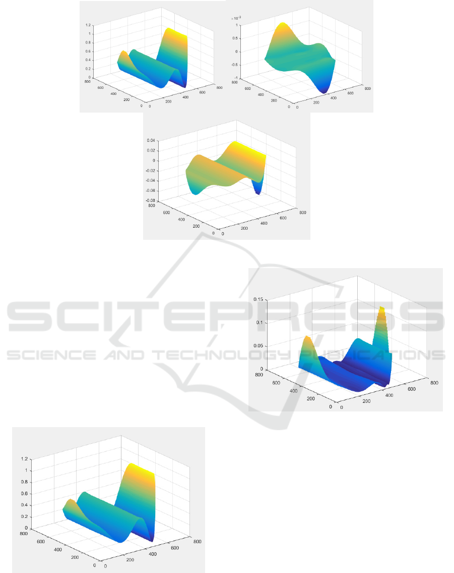
Figure 2: from left: a) test freeform wavefront b) x-slope of wavefront and c) y-slope of wavefront.

The simulation is run using a test freeform

wavefront shown in Figure 2. The test wavefront has

various peaks and valleys and a region of large phase

slope. This would be able to test out and compare both

reconstruction techniques.

The conventional modal wavefront reconstruction

reconstructs the test wavefront relatively well for all

cases. For the case of 317 lenslets, it can be seen that

the reconstructed wavefront retains the overall profile

of the test wavefront from Figure 3. The maximum

error of the reconstructed wavefront is 0.13 microns.

Figure 4 shows the overall absolute error across the

entire phase map.

Figure 3: Reconstructed wavefront using conventional

modal reconstruction (317 lenslet).

Figure 4: Absolute error (in microns).

It can be seen that the highest amount of error is

in the peak region near both ends of the wavefront,

and the lowest valley on the right. The wavefront was

reconstructed using 36 Zernike polynomials. Due to

the limited amount of higher order polynomials, and

the edge being the highest point of the wavefront, the

peak could not be resolved accurately. This occurs for

all the different number of lenslet used. This shows

the limitation in representing phase in the Zernike

domain. Low order Zernike polynomials are very

smooth and are unstable at the outer regions (Dalal, et

al., 2001). Thus they are not very suitable for

freeform wavefronts.

PHOTOPTICS 2016 - 4th International Conference on Photonics, Optics and Laser Technology

156

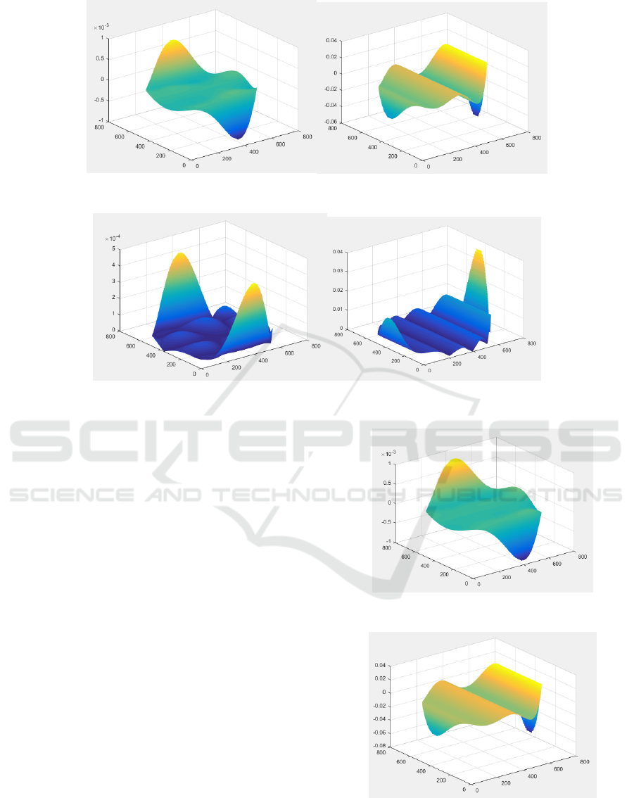
Figure 5: x and y slopes from the reconstructed wavefront.

Figure 6: Absolute error of x and y slopes.

The x and y slopes calculated from the

reconstructed wavefront are shown in Figure 5 and

their error in Figure 6. Again, it can be seen that the

edges have a higher error which is caused by the

inaccuracies in the edges of the reconstructed

wavefront. Discounting the peak at the edges, the

mean error for the x and y slopes are 2.575×10

-5

and

2.649×10

-3

respectively.

SPARZER meanwhile reconstructs the slopes of

the wavefront. The reconstructed slopes using 317

lenslets are shown in Figure 7 and 8, while the

absolute error of the reconstructed slopes are in

Figure 9. Similar to the slope errors from the modal

reconstruction, the largest errors are at the edges

where the slopes are larger in value. Discounting the

peak values at the edges, the mean error for x and y

slopes reconstructed are 2.6346×10

-6

and 2.042×10

-4

respectively.

Table 1 shows the mean error of x and y slopes

obtained using compressed sensing and modal

reconstruction. From the table, it can be seen that

compressed sensing has a lower mean error when

compared to modal reconstruction for all cases.

Figure 7: x-slope reconstructed with SPARZER.

Figure 8: y-slope reconstructed with SPARZER.

Investigation on Compressed Wavefront Sensing in Freeform Surface Measurements

157

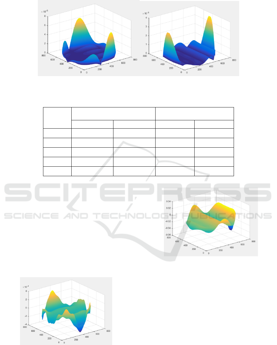
Figure 9: Absolute error of x and y slopes reconstructed with SPARZER.

Table 1: Mean error of wavefront slopes.

No.

lenslets

mean error for compressed

sensing

mean error for modal

reconstruction

x-slope y-slope x-slope y-slope

317

2.63

×10

-6

2.04×10

-6

4.12×10

-5

5.21×10

-3

197

8.59

×10

-6

3.53×10

-6

4.18×10

-5

5.24×10

-3

149

9.84

×10

-6

1.09×10

-5

4.21×10

-5

5.26×10

-3

113

1.31

×10

-5

1.30×10

-4

4.21×10

-5

5.26×10

-3

2.43

×10

-5

5.68×10

-4

4.20×10

-5

5.25×10

-3

Besides that, the mean error for compressed

sensing when using the lowest number of lenslet is

lower than the mean error for all cases using modal

reconstruction. The error from compressed sensing

follows the trend where the higher the number of

samples, the lower the error. Meanwhile for modal

reconstruction, the error stays relatively constant.

However, while the mean errors are lower, the

slopes reconstructed using 81 lenslets do not match

well with the original slopes visually. Shown in

Figure 10 are the slopes reconstructed using 81

lenslets.

Figure 10: x-slope reconstructed with SPARZER.

Figure 11: y-slope reconstructed with SPARZER.

The profile at the edges deviate the most when

compared to the original slopes of the wavefront. This

is again due to the limitations of Zernike polynomials

in freeform surface measurements.

4 CONCLUSIONS

It can be seen that at lower lenslet resolutions, there

are large deviations in the edges of the slopes

reconstructed by compressed sensing. This is caused

by the inability of Zernike polynomials to accurately

represent freeform surface profiles. Similarly, for

modal wavefront reconstruction, the error is also

highest at the edges of the wavefront. However, it is

PHOTOPTICS 2016 - 4th International Conference on Photonics, Optics and Laser Technology

158

clear that compressed sensing yields a lower error

when compared to modal reconstruction for all lenslet

resolutions.

ACKNOWLEDGEMENT

The authors gratefully acknowledge the support and

funding from Monash University Malaysia and

Ministry of Higher Education, Malaysia under the

Grant No: FRGS/1/2013/SG02/MUSM/02/1.

REFERENCES

Basden, A. G., Morris, T. J., Gratadour, D. & Gendron, E.,

2015. Sensitivity improvements for Shack-Hartmann

wavefront sensors using total variation minimization.

Monthly Notices of the Royal Astronomical Society,

Volume 449, pp. 3537-3542.

Candes, E. J. & Romberg, J., 2005. Quantitative Robust

Uncertainty Principles and Optimally Sparse

Decompositions. Classical Analysis and ODEs, pp. 1-

25.

Candes, E., Romberg, J. & Tao, T., 2006. Robust

Uncertaunty Principles: Exact Signal Reconstruction

from Highly Incomplete Frequency Information. IEEE

Transactions on Information Theory, 52(2), pp. 489-

509.

Dai, G.-M., 1994. Modified Hartmann-Shack wavefront

sensing and iterative wavefront reconstruction. s.l., s.n.

Dalal, S., Klein, S., Barsky, B. & Corzine, J. C., 2001.

Limitations to the Zernike representation of cornea and

wavefront for post-refractive surgery eyes, (ARVO

avstract). Investigative Ophtalmology and Visual

Science, 42(4), p. S603.

Donoho, D. L., 2006. Compressed Sensing. IEEE

Transactions on Information Theory, 52(4), pp. 1289-

1306.

Guo, W. et al., 2013. Adaptive centroid-finding algorithm

for freeform surface emasurements. Applied Optics,

52(10), pp. D75-D83.

Hosseini, M. & Michailovich, O. V., 2009. Derivative

Compressive Sampling with Application ti Phase

Unwrapping. Glasgow, s.n.

Lundstrom, L. & Unsbo, P., 2004. Unwrapping Hartmann-

Shack Images from Highly Aberrated Eyes Using and

Iterative B-Spline Based Extrapolation Method.

Optometry and Vision Science, 18(5), pp. 383-388.

Noll, R. J., 1976. Zernike polynomials and atmospheric

turbulence. Optical Society of America, Volume 66, pp.

207-211.

Platt, B. C. & Shack, R., 2001. History and Principles of

Shack-Hartmann Wavefront Sensing. Joirnal of

Regractive Surgery, Volume 17, pp. 573-577.

Polans, J., McNabb, R. P., Izatt, J. A. & Farsiu, S., 2014.

Compressed Wavefront Sensing. Optics Letters, 39(5),

pp. 1189-1192.

Rostami, M., Michailovich, O. & Wang, Z., 2012. Image

Deblurring Using Derivative Compressed Sensing for

Optical Imaging Application. IEEE Transactions on

Image Processing, 21(7), pp. 3139-3149.

Schwiegerling, J. & Neal, D. R., 2005. Historical

Development of the Shack-Hartmann Wavefront

Sensor. Robert Shannon and Roland Shack: Legends in

Applied Optics, pp. 132-139.

Yin, X., Li, X., Zhao, L. & Fang, Z., 2009. Automatic

centroid detection for Shack-Hartmann Wavefront

sensor. s.l., s.n.

Investigation on Compressed Wavefront Sensing in Freeform Surface Measurements

159