
Transductive Transfer Learning to Specialize a Generic Classifier
Towards a Specific Scene
Houda Ma
ˆ
amatou
1,2,3
, Thierry Chateau
1
, Sami Gazzah
2
, Yann Goyat
3
and Najoua Essoukri Ben Amara
2
1
Institut Pascal, Blaise Pascal University, 24 Avenue des Landais, Clermont Ferrand, France
2
SAGE ENISo, University of Sousse, BP 264 Sousse Erriadh, Sousse, Tunisia
3
Logiroad, 2 Rue Robert Schuman, Nantes, France
Keywords:
Transductive Transfer Learning, Specialization, Generic Classifier, Pedestrian Detection, Sequential Monte
Carlo Filter (SMC).
Abstract:
In this paper, we tackle the problem of domain adaptation to perform object-classification and detection tasks in
video surveillance starting by a generic trained detector. Precisely, we put forward a new transductive transfer
learning framework based on a sequential Monte Carlo filter to specialize a generic classifier towards a specific
scene. The proposed algorithm approximates iteratively the target distribution as a set of samples (selected
from both source and target domains) which feed the learning step of a specialized classifier. The output
classifier is applied to pedestrian detection into a traffic scene. We have demonstrated by many experiments,
on the CUHK Square Dataset and the MIT Traffic Dataset, that the performance of the specialized classifier
outperforms the generic classifier and that the suggested algorithm presents encouraging results.
1 INTRODUCTION
In the last fifteen years, we have seen many generic
object detectors which perform detection in static
images; we cite mainly the Viola-Jones detector
(Viola and Jones, 2001) and the HOG-SVM Detector
proposed by Dalal and Triggs (Dalal and Triggs,
2005). However, object detection and classification
on a specific video surveillance scene are still two
interesting and challenging tasks in computer vision
because the algorithm needs to find objects in spite
of their scale and position in the video’s frame, as
well as other variation factors like illumination and
occlusions. In addition, a generic training dataset
contains all possible appearances of the object in
different views and a significant number of negative
images that can not be useful for a specific scene,
which has a unique static background and contains
objects with only a few views. This diversity of
object views and/or of background class leads to weak
performances of a generic detector in a particular
scene.
As a solution to these problems, Transfer Learning
(TL) approaches (also referred to as cross-domain
adaptation approaches) have shown interesting results
by using knowledge from the source domains to learn
a classifier/detector for the target domain containing
unlabelled data or only a few labelled samples.
Pan and Yang (Pan and Yang, 2010) conducted a
survey, providing valuable references for interested
readers. Their work gave the main differences
between the static learning system and the transfer
learning one. Also, they presented the TL works in
three types: inductive, transductive and unsupervised.
The inductive type supposes the presence of some
labelled samples in the target domain. Whereas, the
transductive type deals with a target domain without
any labelled data and assumes that the distribution of
the source domain is different from the target one,
though they are actually related. The unsupervised
type handles unlabelled data into both source and
target domains. The two first types are more presented
in the literature. The transductive TL type allows
avoiding data labelling in each scene and offers
improving object detection/classification in different
videos. These were the reasons that motivate us
to suggest an original formalization of transductive
transfer learning based on a sequential Monte Carlo
filter (Doucet et al., 2001) in order to specialize a
generic classifier to a target domain.
Maâmatou, H., Chateau, T., Gazzah, S., Goyat, Y. and Amara, N.
Transductive Transfer Learning to Specialize a Generic Classifier Towards a Specific Scene.
DOI: 10.5220/0005725104110422
In Proceedings of the 11th Joint Conference on Computer Vision, Imaging and Computer Graphics Theory and Applications (VISIGRAPP 2016) - Volume 4: VISAPP, pages 411-422
ISBN: 978-989-758-175-5
Copyright
c
2016 by SCITEPRESS – Science and Technology Publications, Lda. All rights reserved
411
Prediction
Update
Target dataset
Source dataset
-
-
-
-
-
-
-
-
-
-
+
+
+
+
+
+
+
+
+
+
+
+
+
+
+
+
-
-
-
-
-
-
-
-
-
-
-
-
+
+
+
+
+
+
+
+
+
+
+
+
-
-
-
-
-
-
-
-
-
-
-
-
K0
Generic
classifier
Sampling
Yes
No
K=0 ?
-
-
-
-
-
-
-
-
-
+
+
+
+
Prediction
Update
+
+
+
+
+
+
+
+
+
+
+
+
-
-
-
-
-
-
-
-
-
-
-
-
Kk+1
Sampling
-
-
-
-
-
-
-
-
-
+
+
+
+
-
-
-
Specialized dataset
Stopping
criteria
Yes
No
-
-
-
-
- -
+
+
+
-
-
-
-
- -
+
+
+
+
+
+
+
+
+
+
+
+
+
+
+
-
-
-
-
-
-
-
-
-
-
-
-
Subset-2
Subset-1
Yes
Specialized classifier
Output
-
-
-
-
-
- -
-
-
-
+
+
+
+
Specialized dataset
Intermediate result
Legend:
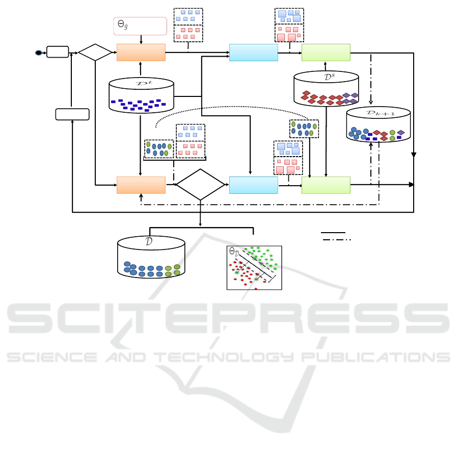
Figure 1: A synthetic block diagram of the proposed approach. The unknown target distribution is approximated through a
sequential Monte-Carlo algorithm.
This filter selects training dataset samples that are
considered to be realizations of the joint probability
distribution between features’ samples and object
classes corresponding to the target scene.
Figure 1 shows the block diagram of our approach
which aims to estimate the hidden distribution of the
target dataset through a set of iterations. At the first
iteration, a generic classifier is used to predict a set of
samples from the target dataset. Then, the update step
determines the relevance of each samples by using an
observation function. After that, the sampling step
proposes the first specialized dataset from target and
source samples. The observation function utilizes
widely information which is extracted from the target
scene. This is close to Wang’s (Wang et al., 2012a)
visual cues and those used by Chesnais (Chesnais
et al., 2012).
The process is the same at a different iteration,
but the prediction step uses a specialized classifier,
trained on a dataset built at the previous iteration, to
propose new samples belonging to the target dataset.
The sampling step draws a new training dataset from:
1) the previous specialized dataset, 2) the target
dataset and 3) a source dataset to approximate the
target distribution.
In this paper, our main contributions are:
• Proposing an original formalization of transfer
learning for the specialization of a generic
classifier to a target domain;
• Applying our algorithm to detect pedestrians in
traffic video sequences;
• Evaluating our proposed method to the state of the
art on two public datasets.
The next section gives some related works.
Section 3 describes the proposed approach. Section
4 presents a pedestrian detection framework as an
application of the method to validate our concepts.
Our experiments and results are provided in section
5. The last section is a conclusion and gives some
perspectives.
2 RELATED WORKS
In this section we describe three categories of
transfer learning works which provide specific
detectors/classifiers to a particular domain. Then,
we are limited to the closest group that suggests to
improve pedestrian detection into a video surveillance
scene, corresponding to the application we present to
validate our specialization framework.
VISAPP 2016 - International Conference on Computer Vision Theory and Applications
412

The first category of TL methods has aimed to
modify the parameters of a source learning model
to improve its functioning in a target domain, as
presented in (Aytar and Zisserman, 2011; Tommasi
et al., 2010; Pang et al., 2011; Dai et al., 2007;
Yang et al., 2007), by leveraging the visual knowledge
of source data or other forms of prior knowledge.
Wang et al.(Wang et al., 2012b) proposed to leverage
a vocabulary tree as a binary vector to encode
visual example for detector adaptation. In addition,
Salakhutdinov et al. (Salakhutdinov et al., 2010) used
a higher-order knowledge abstracted from previously
learned classes to predict the label of a new class by
using only one sample.
The second category of works has dealt with
distribution adaptation to reduce the difference
between source and target domains. For instance, Pan
et al. (Pan et al., 2011) learnt a low-dimensional
space where the distance in marginal distributions
could be reduced. Moreover, Quanz et al. (Quanz
et al., 2012) minimized both marginal and conditional
distributions. In contrast to these two methods, which
expect either the presence of multi- source domains
or labelled target data, Long et al. (Long et al.,
2013) suggested a new approach able to jointly adapt
the marginal and conditional distributions using a
procedure to reduce the dimension of data in both
domains and build a new feature representation that
would fill in the distributions’ difference.
The third category of transfer learning methods
has automatically selected training samples that have
given a better model for the target task. Lim et al.
(Lim et al., 2011) put forward a transfer learning
approach based on borrowing training samples from
similar categories to the target class. Then, they
applied a set of transformations to the borrowed
samples to generate the target dataset. Inspired
from this, Tang et al. (Tang et al., 2012) used a
binary-valued variables to weight examples, which
would be added or excluded from the training set.
In this part, we have focussed on some works
related to pedestrian detection application. This group
is based on using or building an automatic labeller to
collect data from the target domain. Rosenberg et al.
(Rosenberg et al., 2005) utilized the decision function
of an object appearance classifier to select the training
samples from one iteration to another. Levin et
al. (Levin et al., 2003) used a system with two
independent classifiers to collect unlabelled data. The
labelled data with high confidence, by one classifier
or another, were added to the training data to retrain
the two classifiers. Another way to automatically
collect new samples is to use an external entity
called “oracle”. An oracle may be built using a
single algorithm or combine and/or merge multiple
algorithms. In (Nair and Clark, 2004), an algorithm
based on background subtraction was presented.
Also, Chesnais et al. (Chesnais et al., 2012) proposed
an oracle composed of three independent classifiers
(appearance, background extraction, and optical
flow). Furthermore, some solutions concatenate the
source dataset with new samples, which increases the
size of the dataset during iterations. Others are limited
only to the use of new samples, which results in losing
pertinent information of source samples. Another
solution was proposed in (Wang et al., 2012a; Tang
et al., 2012; Zeng et al., 2014; Wang and Wang, 2011;
Wang et al., 2014; Wang et al., 2012b). It collected
new samples from the target domain and selected only
the useful ones from the source dataset. Wang et al.
(Wang et al., 2014) used many contextual cues such as
pedestrian motion, road model (pedestrians, cars ...),
location, size and objects’ visual appearances to select
positive and negative samples of the target domain. In
fact, their method was based on a new SVM variant
to select only source samples that were good for the
classification in the target scene. Zeng et al. (Zeng
et al., 2014) utilized Wang’s approach (Wang et al.,
2014) as an input to their deep model, which learnt the
distribution of target domain and re-weighted samples
from both domains.
Except Zeng et al. (Zeng et al., 2014), all the
latter approaches did not learn or estimate the target
domain distribution. However, our Transductive
Transfer Learning framework based on a Sequential
Monte Carlo (TTL-SMC) aims to approximate
iteratively the joint probability distribution between
the feature descriptors’ samples and the object classes
corresponding to the target scene. This is done by
using the Sampling Importance Resampling (SIR)
algorithm (Doucet et al., 2001) to select both target
and source samples according to the output of an
observation function and a visual similarity weighting
procedure.
3 CLASSIFIER SPECIALIZATION
BY A SEQUENTIAL MONTE
CARLO FILTER
This section describes the core of the proposed
specialization method done by a transfer learning
approach based on a sequential Monte Carlo filter.
Transductive Transfer Learning to Specialize a Generic Classifier Towards a Specific Scene
413
3.1 Context
Let us have a source dataset, a generic detector –
which can be learnt from this source dataset – and
a video sequence of a target scene. A specialized
classifier and an associated specialized dataset are to
be generated. A huge number of unlabelled samples
can be generated from the target video.
We assume that the unknown jointed distribution
between the target features and the associated class
labels can be approximated by a set of well chosen
samples. This latter can be used as a specialized
training dataset. We propose to approximate this
distribution by a sequential Monte Carlo filter.
Let D
k
.
= {X
(n)
k
}
n=1,..,N
be a specialized dataset of
size N at an iteration k, where X
(n)
k
.
= (x
(n)
,y) is the
sample number n, with x being its feature vector, and
y is its label, with y ∈ Y . Basically, in a detection
case, Y = {−1;1}, where 1 represents the object
and −1 represents the background (or non-object
class). In addition, Θ
D
k
is a specialized classifier at an
iteration k, which is trained on the specialized dataset
built at the previous iteration (k − 1). A classifier
assigns a label y to a feature vector x. We have used a
generic classifier Θ
g
at the first iteration.
A source dataset D
s
.
= {X
s(n)
}
n=1,..,N
s
of N
s
labelled samples is defined. Moreover, a large target
dataset D
t
.
= {x
t(n)
}
n=1,..,N
t
is available. This dataset
is composed of N
t
unlabelled samples provided by a
multi-scale sliding window extraction strategy on the
target video sequence.
3.2 Sequential Monte Carlo Filter
The suggested transfer learning algorithm is based
on the assumption that the target distribution can
be approximated by the samples of the specialized
dataset. These samples are initially unknown but they
can be estimated using an observation process and
some prior information from the target scene.
We define X
k
a hidden state associated to an
unknown sample at an iteration k and Z
k
an
observation extracted from the target video sequence.
Based on our assumption, the target distribution can
be approximated by iteratively applying equation (1):
p(X
k+1
|Z
0:k+1
) =
C.p(Z
k+1
|X
k+1
)
Z
X
k
p(X
k+1
|X
k
)p(X
k
|Z
0:k
)dX
k
(1)
where C = 1/p(Z
k+1
|Z
0:k+1
).
The sequential Monte Carlo method approximates
the posterior distribution p(X
k
|Z
k
) by a set of N
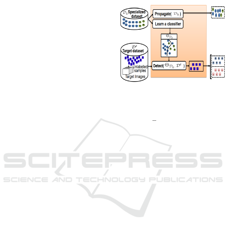
Figure 2: Details of the prediction step processing.
particles (samples in this case), according to equation
(2):
p(X
k
|Z
k
) ≈
1
N
N
∑
n=1
δ(X
(n)
k
) ≈ {X
(n)
k
}
n=1,..,N
(2)
Therefore, a sequential Monte Carlo filter is used
to estimate the unknown jointed distribution between
the features of the target samples and the associated
class labels. We suppose that the recursion process
selects relevant samples for the specialized dataset
from one iteration to another, which leads to converge
to the right target distribution and which makes the
resulting classifiers more and more efficient.
The resolution of equation (1) is done in three
steps: prediction, update and sampling. These steps
are the same as those into the particle filter used,
in general, to solve tracking problems in computer
vision (Isard and Blake, 1998; Smal et al., 2007; Mei
and Ling, 2011). An illustration of our proposed
algorithm is shown in Figure 1 and the details of
the three main steps are described in the following
subsections.
3.2.1 Prediction Step
Figure 2 shows an overview of the prediction step
processing at a given iteration. This step consists in
applying the Chapman-Kolmogorov equation (3):
p(X
k+1
|Z
0:k
) =
Z
X
k
p(X
k+1
|X
k
)p(X
k
|Z
0:k
)dX
k
(3)
It uses the term p(X
k+1
|X
k
) of the system
dynamics between two iterations to propose a
specialized dataset D
k
.
= {X
(n)
k
}
n=1,..,N
s
producing the
approximation (4):
p(X
k+1
|Z
0:k
) ≈ {
˜
X
(n)
k+1
}
n=1,..,
˜
N
k+1
(4)
VISAPP 2016 - International Conference on Computer Vision Theory and Applications
414
We note
˜
D
k+1
the specialized dataset predicted for an
iteration (k + 1) where
˜
X
(n)
k+1
is the predicted sample
n and
˜
N
k+1
is the number of samples provided by the
prediction step. In our case, this predicted dataset is
composed of two subsets:
1. Subset 1: It corresponds to sub-sampling the
previous specialized dataset to propagate the
distribution. The ratio between the positive
and negative classes (typically the same as the
source dataset) should be respected. This subset
approximates the term p(X
k
|Z
0:k
) in equation (1),
according to equation (5):
p(X
k
|Z
0:k
) ≈ {X
∗(n)
k+1
}
n=1,..,N
∗
(5)
where X
∗(n)
k+1
is the sample n selected from D
k
to be in the dataset of the next iteration (k + 1)
and N
∗
represents the number of samples in this
subset with N
∗
= α
t
N
s
, where α
t
∈ [0,1]. The
parameter α
t
determines the number of samples
to be propagated from the previous dataset.
2. Subset 2: It is a part of target samples selected as “
positive ” by a classifier trained on D
k
and applied
on the target dataset D
t
. This subset contains
several samples which are not really positive, in
particular at the first iteration where we use a
generic classifier that gives a weak result.
At this step, all samples returned by (6) are
supposed to be both positive and negative and the
decision between the two labels will be provided
by the observation function in the update step.
{
˘
X
(n)
k+1
}
n=1,..,
˘
N
k
.
=
{(x
(n)
,y)}
y∈Y ;x
(n)
∈D
t
/Θ
D
k
(x
(n)
)>0
(6)
˘
X
(n)
k+1
is the n
th
target sample proposed to be
included in the dataset of the next iteration (k +1).
Initially, this subset has been classified positive by
Θ
D
k
.
In what follows, we note the functions returning these
two subsets by Propagate(D
k
) and Detect(Θ
D
k
,D
t
),
respectively.
3.2.2 Update Step
The update step assigns a weight
˘
π
(n)
k+1
to each sample
˘
X
(n)
k+1
returned by the function Detect(Θ
D
k
,D
t
) to
define the likelihood term (7) by using an observation
function.
p
Z
k+1
|X
k+1
=
˘
X
(n)
k+1
∝
˘
π
(n)
k+1
(7)
The observation function uses visual contextual cues
and prior information extracted from the target video
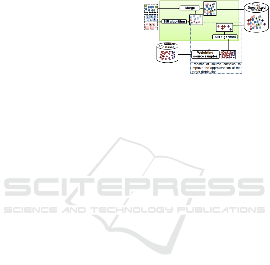
Figure 3: Details of the sampling step.
sequence like object motion, background subtraction
and/or object path model, which are used extensively
in the state of the art. The output of this step is a set
of weighted target samples, which will be referred to
as “the weighted target dataset” hereafter (8):
{(
˘
X
(n)
k+1
,
˘
π
(n)
k+1
)}
n=1,..,
˘
N
k+1
(8)
where (
˘
X
(n)
k+1
,
˘
π
(n)
k+1
) represents a target sample and its
associated weight and
˘
N
k+1
is the number of samples
that have a weight different from zero.
3.2.3 Sampling Step
The sampling step in our case determines exactly
which samples would be included in the specialized
dataset for the next iteration. Figure 3 illustrates
the details about this step. On the one hand, we
use the SIR algorithm to generate a new set of
unweighted target samples from the weighted target
dataset provided by the update step. This last
weighted target dataset approximates the conditional
distribution p(
˘
X
k+1
|Z
k+1
) of the target samples given
by the observations. After applying the SIR, we have
a set of target samples that approximate the same
distribution (9):
p(
˘
X
k+1
|Z
k+1
) ≈ {
˘
X
∗(n)
k+1
}
n=1,..,
˘
N
∗
k+1
(9)
where
˘
X
∗(n)
k+1
is the selected sample n for the next
iteration (k +1) from the weighted target dataset.
At this level, the posterior distribution
p(X
k+1
|Z
0:k+1
) is approximated by (10):
p(X
k+1
|Z
0:k+1
) ≈ {X
∗(n)
k+1
}
n=1,..,N
∗
∪{
˘
X
∗(n)
k+1
}
n=1,..,
˘
N
∗
k+1
(10)
On the other hand, we propose to utilize the
source distribution to improve the estimation of the
target one. The new specialized dataset is extended
by transferring samples from the source dataset
without changing the posterior distribution. The
probability that each source sample belongs to the
Transductive Transfer Learning to Specialize a Generic Classifier Towards a Specific Scene
415

Table 1: Functions and notations used in this paper.
Notation: definition
-Detect(Θ
D
k
,D
t
): applies a classifier Θ
D
k
on
the target dataset D
t
to predict a set of samples.
-Propagate(D
k
): selects samples to propagate
from D
k
to D
k+1
.
- Lear n(Θ, D): learns a classifier Θ on
the dataset D.
- Obs f n: the observation function.
- p: is a spatio-temporal Region Of Interest (ROI)
position into the target video-sequence (D
t
).
- compute overlap(p, D
t
): computes an
overlap score of ROI p.
- compute accumulation(p,D
t
): computes an
accumulation score of ROI p
target distribution p(X
k+1
|Z
0:k+1
) is estimated from
the current set of target samples by a non parametric
method (KDE or KNN estimator). Based on these
probabilities, we apply the SIR algorithm to select
the source samples that approximate p(X
k+1
|Z
0:k+1
)
according to equation (11) :
p(X
k+1
|Z
0:k+1
) ≈ {X
s∗(n)
k+1
}
n=1,..,
˘
N
s∗
k+1
(11)
where X
s∗(n)
k+1
is the source sample n selected to be
in the specialized dataset at the iteration (k + 1) and
˘
N
s∗
k+1
is the number of the selected source samples.
This number is determined using equation (12):
˘
N
s∗
k+1
= N
s
− (N
∗
+
˘
N
∗
k+1
) (12)
Finally, the new dataset for the iteration (k +1) is built
by the union of three subsets (13):
D
k+1
.
= {X
∗(n)
k+1
}
n=1,..,N
∗
∪
{
˘
X
∗(n)
k+1
}
n=1,..,
˘
N
∗
k+1
∪ {X
s∗(n)
k+1
}
n=1,..,
˘
N
s∗
k+1
(13)
The process stops when the ratio (|
˜
D
k+1
|/|
˜
D
k
|)
(| • | represents the dataset cardinality.) exceeds a
previously determined threshold α
s
.
Table 1 defines the functions and notations that
are used in the rest of the paper, and Algorithm 1
describes the TTL SMC process.
4 APPLICATION TO
PEDESTRIAN DETECTION
This section presents an application of our TTL-SMC
framework to specialize a generic detector to a
specific traffic scene which ameliorates pedestrian
detection with an automatic labelling of target data.
In the following sub-sections, the three stages of
the proposed algorithm are presented.
Algorithm 1: Transfer learning for specialization.
Input: Source dataset D
s
Generic classifier Θ
g
Target video scene and the associated dataset D
t
Number of source samples N
s
.
The parameter α
t
, α
s
.
Output: The last specialized dataset D
The last classifier Θ
D
———————————————————
k ← 0
stop ← f alse
while stop 6= true do
if (k = 0) then
/* Prediction step */
N
∗
← 0
˜
D
k+1
← Detect(Θ
g
,D
t
)
/* Update step */
{(
˘
X
(n)
k+1
,
˘
π
(n)
k+1
)}
n=1,..,
˘
N
k+1
← Obs f n
/* Sampling step */
D
k+1
← {
˘
X
∗(n)
k+1
}
n=1,..,
˘
N
∗
k+1
∪{X
s∗(n)
k+1
}
n=1,..,
˘
N
s∗
k+1
else
/* Prediction step */
Learn (Θ
D
k
,D
k
)
N
∗
← α
t
N
s
˜
D
k+1
← Propagate(D
k
) ∪ Detect(Θ
D
k
,D
t
)
if (|
˜
D
k+1
|/|
˜
D
k
| >= α
s
) then
stop ← true
Break
end if
/* Update step */
{(
˘
X
(n)
k+1
,
˘
π
(n)
k+1
)}
n=1,..,
˘
N
k+1
← Obs
f n
/* Sampling step */
D
k+1
←equation (13)
end if
k ← k + 1
end while
4.1 Prediction Step
The prediction step consists in selecting randomly a
set of samples (subset 1) from the specialized dataset
of the previous iteration. In addition, a second set
of detection proposals (subset 2) is provided by a
detector trained on the previous specialized dataset
and applied on the target video-sequence, using a
multi-scale sliding windows strategy.
This strategy provides a set of samples that were
classified by the classifier as pedestrian, but really
there are both true and false detections (Figure 4).
A spatial mean-shift is applied to merge the closest
detections. Herein, we suppose that each detection of
subset 2 can be either a positive sample or a negative
one. Thus, each detection produces both a positive
VISAPP 2016 - International Conference on Computer Vision Theory and Applications
416
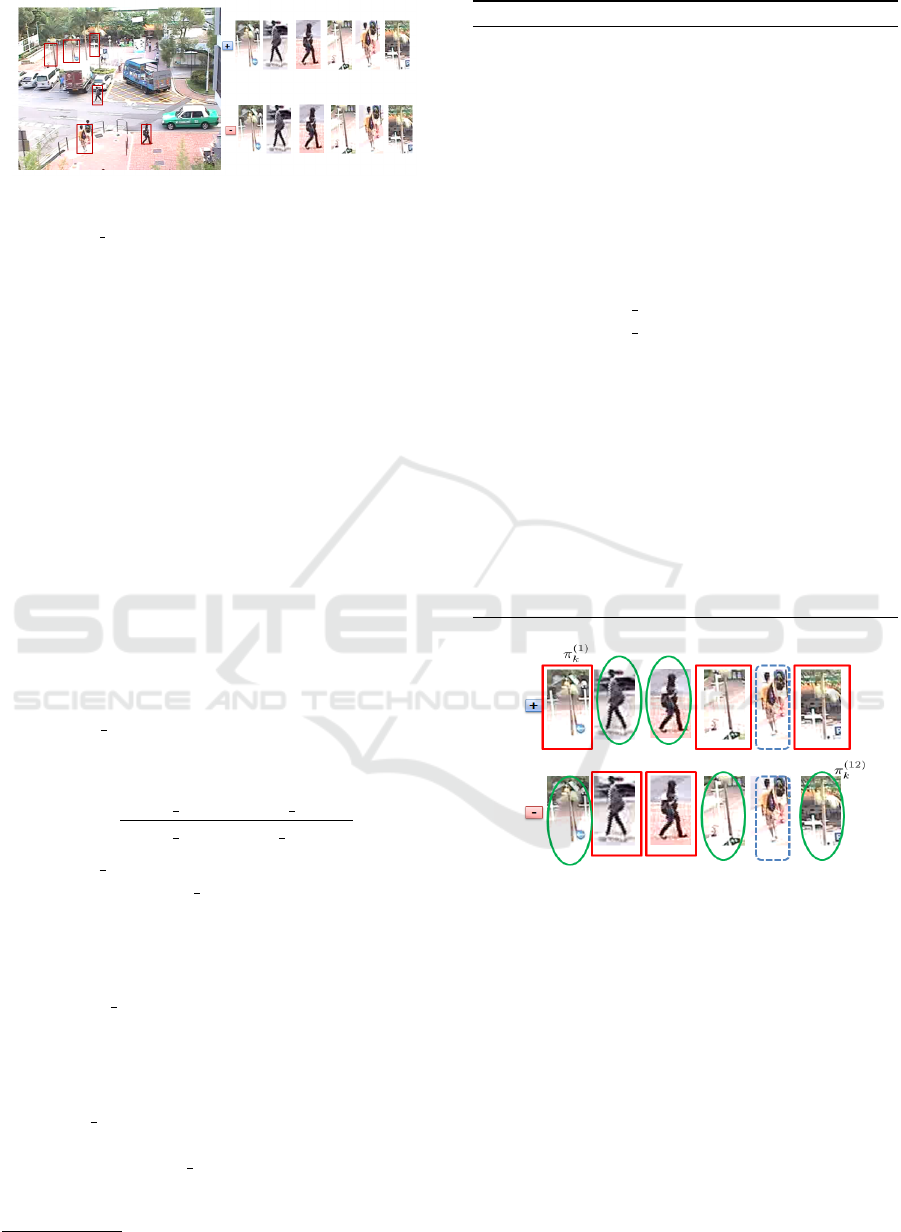
Figure 4: Illustration of the prediction step result:
Detections provided by a generic detector applied on frames
of the CUHK Square dataset.
sample and a negative one.
At the first iteration, it is to note that subset 1
is empty and that proposals composing subset 2 are
given from a generic detector trained on the INRIA
Person Dataset, in a similar way to the one proposed
by Dalal and Triggs in (Dalal and Triggs, 2005).
In our application, we have trained the generic and
the specialized classifiers using the SVMLight
1
.
4.2 Update Step
This step computes a weight for each sample of
“subset 2” using an observation function. This
likelihood function is based on visual cues. We
put forward two simple spatio-temporal cues: a
background extraction overlap score and a temporal
accumulation score.
We assume that pedestrians are moving and
that a good detection occurs on a foreground blob.
The overlap score λ
o
(14) compares the Region Of
Interest (ROI) associated to one sample with the
output of a binary foreground extraction algorithm.
λ
o
.
=
2(ROI AREA × FG AREA)
ROI AREA + FG AREA
(14)
where ROI AREA is the area in pixels of the
considered ROI and FG AREA is the foreground area
at the ROI position.
Additionally, false positive detections on
background provide some ROIs that temporally
“twinkle” on the target video-sequence. An
accumulation score λ
a
is computed in order to detect
such hard background regions, where the detector
responds positively.
The observation function (Algorithm 2) assigns
a high weight to a positive proposition if it has
an overlap score λ
o
that exceeds a fixed threshold
α
p
, which is determined empirically. On the other
hand, the accumulation score gives information about
negative propositions. A negative sample which
has a big score λ
a
can be a correct proposition;
1
http://svmlight.joachims.org
Algorithm 2: Observation function.
Input: Subset-2 {
˘
X
(n)
k+1
}
n=1,..,
˘
N
with associated ROI
position and size {p
i
}
i=1,..,
˘
N
into the target
video-sequence
Target video sequence and associated dataset D
t
α
p
: overlap threshold
Output: Set {π
i
}
i=1..,L
of weights associated to
samples
———————————————————–
for i = 1 to L do
π
i
← 0
/* Visual contextual cues computation */
λ
o
← compute overlap(p
i
,D
t
)
λ
a
← compute accumulation(p
i
,D
t
)
/* Weight assignment */
if ( ˘y
i
= pedestrian) then
if (λ
o
> α
p
) then
π
i
← λ
o
end if
else
if ((λ
o
= 0.0)&(λ
a
> 0.0)) then
π
i
← λ
a
end if
end if
end for
Figure 5: The observation function result at the iteration
k: The assigned weight allows privileging one label from
the two propositions. A green ellipse means the sample
is correct according to the proposed label, a red rectangle
means that the proposed label is not correct and a blue
dotted rectangle means that the sample should be rejected.
i.e., it should have a high weight (an example of
the observation function result is shown in Figure
5). Negative propositions are called “hard-examples”
because they are classified by the previous detector
as pedestrians, but currently they are not. The use of
these samples in the next specialized dataset improves
the performance of the specialized classifier. After
applying algorithm 2, any proposition that has a null
weight will be rejected.
Transductive Transfer Learning to Specialize a Generic Classifier Towards a Specific Scene
417

4.3 Sampling Step
This step aims to select target and source samples in
order to build a specialized dataset that approximates
the target distribution.
The update step provides a weighted target
dataset approximating the target distribution. A SIR
algorithm is applied to build an unweighted target
dataset which has the same number of samples as the
weighted one.
The resulting dataset approximates the target
distribution. In order to extend this dataset without
altering the latter distribution, we propose to draw
samples from the source dataset. The probability
(weight) that each source sample belongs to the target
distribution
˘
π
s(n)
k+1
is computed using a non-parametric
method based on the KNN algorithm (using the
FLANN
2
library and an L2 distance on features). The
SIR algorithm is used in order to select the source
samples to be included in the specialized dataset. As
the weights used in the SIR algorithm are proportional
to the probability that a sample should derive from
the target distribution, the resulting distribution is the
same as the target one.
At the end of this step, three subsets are merged to
produce the new specialized dataset: the propagated
selection from the previous dataset, the unweighted
target dataset and the new source dataset resulting
from the SIR algorithm.
The specialization process stops when the ratio
α
s
is reached (α
s
= 0.80 fixed empirically in our
case). Once the specialization is finished, the obtained
detector can be used for pedestrian detection in the
target scene based only on appearance.
5 EXPERIMENTS AND RESULTS
This section presents the experiments achieved in
order to evaluate the specialization’s performances.
We have tested our method on two public traffic
videos using the same setting as in (Wang and Wang,
2011; Wang et al., 2012a; Wang et al., 2014; Zeng
et al., 2014).
• The CUHK Square Dataset (Wang et al.,
2012a): It is a video sequence of road traffic
which takes 60 minutes. We have used 352
images for the specialization, which have been
extracted uniformly from the first half of the
video. We have used for the test 100 images,
which have been extracted from the second 30
minutes.
2
http://www.cs.ubc.ca/research/flann/
• The MIT Traffic Dataset (Wang et al., 2009): It
is a set of 20 short video sequences of a 90-minute
video all in all. We have used 420 images
for the specialization, which have been extracted
uniformly from the 10 first videos. Also, 100
images are extracted from the second 10 videos
for the test.
To evaluate the detection results of our specialized
detectors on the CUHK
Square dataset and on the
MIT Traffic dataset, we have used the ground truth
provided by Wang et al. in (Wang et al., 2012a) and
(Wang and Wang, 2011), respectively. The PASCAL
rule (Everingham et al., 2010) is applied to calculate
the rate of the true positives. A detection is considered
good if the overlap area between the detection
window and the ground truth exceeds 0.5 of the union
area. The detection performances are compared using
the Receiver Operating Characteristic (ROC) curve,
presenting the pedestrian detection rate for a given
false positive rate per image.
In the following sub-sections, the indication of a
detection’s rate is always related to one False Positive
Per Image (FPPI=1). We first discuss the convergence
of the specialization algorithm and the influence of
the number of propagated samples (the parameter α
t
)
on the detection performances. Then, we compare the
proposed algorithm with the state of the art methods
on two public datasets.
5.1 Convergence of Specialized Detector
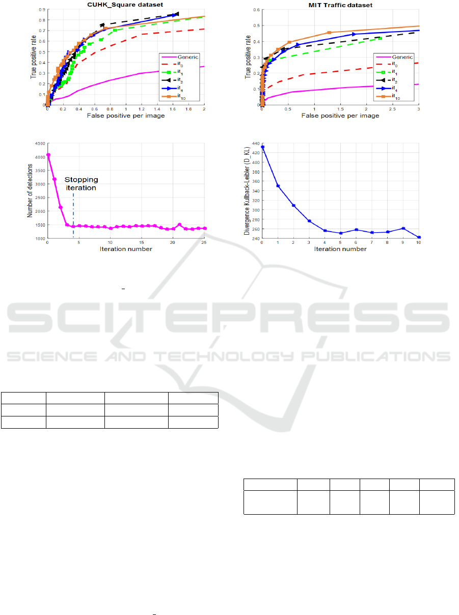
Figures 6 (a) and (b) compare the performance
of the specialized detector at several iterations to
the performance of the generic detector, on the
CUHK Square dataset and the MIT Traffic dataset,
respectively. They show that the specialized detector
trained by our TTL-SMC generates an increase in
the detection rate from the first iteration. On
the CUHK Square dataset, the specialized detector
performance exceeds that of the generic one by more
than 30% and the curves show that the specialization
converges after four iterations with a rate of true
positives higher than 70%. On the MIT Traffic
dataset, our framework improves the detection rate
from 10% to 20% and it starts converging from the
fourth iteration with 40% of true detections. The
experiments demonstrate that the performance has
improved weakly for the next five iterations (for
clarity reasons, we have limited the visualization of
the ROC at the tenth iteration) taking into account
the average duration needed for selecting samples and
training the specialized detector. Table 2 reports the
average duration of a specialization’s iteration on a
machine Intel(R) Core(TM) i7- 3630QM 2.4G CPU
VISAPP 2016 - International Conference on Computer Vision Theory and Applications
418
(a) (b)
(c) (d)
Figure 6: Convergence evaluation: (a) & (b) Comparison between the generic detector and the specialized detectors through
several iterations, on the CUHK Square dataset and the MIT traffic dataset, respectively. (c) Number of detections during
iterations; it converges after the fourth iteration. (d) Divergence Kullback-Leibler between the positive samples of the
specialized datasets for the first ten iterations and the true manually labelled positive samples of the specialization images.
to apply the detection and the observation function
on each dataset with the designed number and size
of images.
Table 2: Average duration of a specialization’s iteration on
the two datasets.
Dataset Nb. images Image size Duration
CUHK 352 1440 × 1152 1 hour
MIT 420 4320 × 2880 3.5 hours
In addition to these latter considerations, we
have noticed that the number of detections stabilizes
from iteration 4, which corresponds to the stop
iteration according to the stopping criterion α
s
,
defined previously (Figure 6-(c)).
In order to measure whether the estimated
distribution converges toward the true target
distribution, we have manually cropped samples to
build a target labelled dataset. The Kullback-Leibler
Divergence (KLD) has been computed between the
specialized dataset, produced at each iteration, and
the ground truth target dataset. Figure 6-(d) shows
that the KLD decreases until having a minimal
variation starting from iteration 4 (corresponding to
the stopping iteration) on the CUHK Square dataset.
The recorded decrease in the KLD explains the
convergence of the specialization process to the true
target distribution.
5.2 Influence of Parameter α
t
The parameter α
t
is used to adjust the number of
samples that propagate from one iteration to another.
Table 3 shows the performances of detectors with
different values of α
t
. It presents a maximal detection
rate, which is equal to 77%, corresponding to the
value of 0.75.
Table 3: Detection rate of different detectors for various
values of parameter α
t
relative to FPPI=1.
α
t
0.1 0.25 0.5 0.75 0.9
Detection
67.2 70.2 73.9 77 75.38
rate (%)
5.3 Comparaison with State of the Art
Algorithms
The overall performance of our method has been
compared with the following methods of the state of
the art:
• Generic (Dalal and Triggs, 2005): A detector
has been created in a similar way, as proposed
Transductive Transfer Learning to Specialize a Generic Classifier Towards a Specific Scene
419
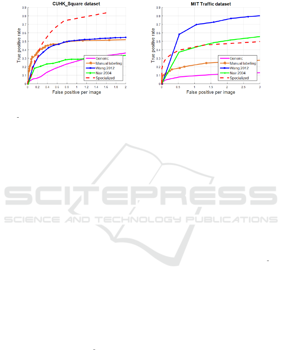
(a) (b)
Figure 7: Overall performance: Comparison of the specialized detector with other methods of the state of the art: (a) on the
CUHK Square dataset, (b) on the MIT traffic dataset.
by Dalal and Triggs and trained on the INRIA
dataset.
• Manual Labelling: A detector has been trained
on a set of labelled samples, cropped from the
target video. This latter has been composed by
all the pedestrians of the specialization’ images
and negative thumbnails that have been randomly
extracted.
• Wang 2012 (Wang et al., 2012a): A specific
target scene detector which has been trained
on both INRIA samples and samples extracted
automatically from the target scene. The
selected target and the INRIA’s samples are
those which have had a high confidence score.
The scores have been calculated using several
contextual cues. The selection of training
samples has been done by a new SVM variant,
called “Confidence-Encoded SVM” which favors
samples with a high score.
• Nair 2004 (Nair and Clark, 2004): A detector
based on an automatic adaptation approach has
selected the target samples to be added in the
initial training dataset using the result of the
background subtraction method. It is a detector
similar to the detector proposed in (Nair and
Clark, 2004) but it has been created with the HOG
descriptor and the SVM classifier.
Figure 7.(a) shows that the specialized detector
significantly exceeds the generic detector on the
selected test images of the CUHK Square dataset.
The performance has improved from 26.6% to
74.37%. The specialized detector exceeds also the
two other detectors of Nair 2004 and Wang 2012,
respectively, by 45.57% and 23.25%. However, the
target detector with manual labelling slightly exceeds
the specialized detector for an FPPI of less than
0.2, but the specialized detector clearly exceeds this
latter for a FPPI that is strictly greater than 0.2. In
particular, it presents an improvement rate equal to
23.25% at FPPI = 1.
On the MIT Traffic dataset (Figure 7.(b)), the
detection rate improves from 10% to 43%. The
specialized detector even outperforms the detector
trained on the target samples, labelled manually, by
about 21%. Compared to Nair 2004’s detector, our
specialized detector gives a better detection rate than
the one proposed by Nair and Clark for an FPPI
less than 1. Otherwise, Nair 2004’s detector slightly
exceeds our specialized detector. Exceptionally,
Wang 2012’s detector outperforms our specialized
detector by about 26%. This can be due to two facts.
First, the MIT Traffic scene is very structured, which
helps Wang et al. to get the most confident samples
by using the cue of path models. Second, the video
presents the shadow that makes our overlap score
unable to determine the correct positive samples.
Figure 8 shows that the specialization has
considerably reduced the number of false detections
and has improved the detection of some non-detected
pedestrians by the generic detector. It demonstrates
also the precise locations of the specialized detector.
6 CONCLUSIONS
In this paper, we have put forward a new transductive
transfer learning method based on a sequential
Monte Carlo filter that selects relevant samples
and estimates the unknown target distribution.
These samples can be used to learn a specialized
classifier that importantly improves the detection
performances. The suggested method has been
validated on a pedestrian detection application using
VISAPP 2016 - International Conference on Computer Vision Theory and Applications
420
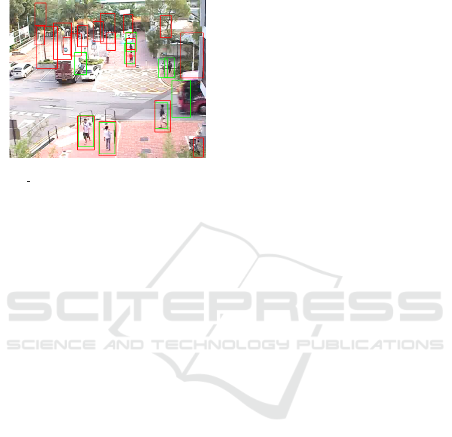
Figure 8: Illustration of the specialization result on the
CUHK Square dataset. The red bounding boxes and the
green bounding boxes present the outputs of the generic and
specialized detector, respectively.
the HOG-SVM classifier. The experiments have
shown that the proposed specialization framework has
good performances from the early iterations on two
public datasets.
Future works will deal with an extension of the
algorithm to a multi-object framework. Furthermore,
the observation function may be ameliorated with
more complex visual cues like tracking, optical flow
or contextual information.
ACKNOWLEDGEMENTS
This work is supported by a CIFRE convention with
the company Logiroad and it has been sponsored
by the French government research programme
”Investissements d’avenir” through the IMobS3
Laboratory of Excellence (ANR-10-LABX-16-01),
by the European Union through the programme
Regional competitiveness and employment
2007-2013 (ERDF Auvergne region), and by
the Auvergne region.
REFERENCES
Aytar, Y. and Zisserman, A. (2011). Tabula rasa: Model
transfer for object category detection. In ICCV, pages
2252–2259. IEEE.
Chesnais, T., Allezard, N., Dhome, Y., and Chateau, T.
(2012). Automatic process to build a contextualized
detector. In VISAPP, volume 1, pages 513–520.
SciTePress.
Dai, W., Yang, Q., Xue, G.-R., and Yu, Y. (2007). Boosting
for transfer learning. In ICML, pages 193–200. ACM.
Dalal, N. and Triggs, B. (2005). Histograms of oriented
gradients for human detection. In CVPR, volume 1,
pages 886–893. IEEE.
Doucet, A., De Freitas, N., and Gordon, N. (2001).
Sequential Monte Carlo Methods in Practice.
Springer.
Everingham, M., Van Gool, L., Williams, C. K., Winn, J.,
and Zisserman, A. (2010). The pascal visual object
classes (VOC) challenge. IJCV, 88(2):303–338.
Isard, M. and Blake, A. (1998). Condensationconditional
density propagation for visual tracking. IJCV,
29(1):5–28.
Levin, A., Viola, P., and Freund, Y. (2003). Unsupervised
improvement of visual detectors using cotraining. In
CV, pages 626–633. IEEE.
Lim, J. J., Salakhutdinov, R., and Torralba, A.
(2011). Transfer learning by borrowing examples for
multiclass object detection. In NIPS.
Long, M., Wang, J., Ding, G., Sun, J., and Yu,
P. S. (2013). Transfer feature learning with joint
distribution adaptation. In ICCV, pages 2200–2207.
IEEE.
Mei, X. and Ling, H. (2011). Robust visual tracking and
vehicle classification via sparse representation. PAMI,
33(11):2259–2272.
Nair, V. and Clark, J. J. (2004). An unsupervised, online
learning framework for moving object detection. In
CVPR, volume 2, pages II–317. IEEE.
Pan, S. J., Tsang, I. W., Kwok, J. T., and Yang, Q. (2011).
Domain adaptation via transfer component analysis.
NN, 22(2):199–210.
Pan, S. J. and Yang, Q. (2010). A survey on transfer
learning. KDE, 22(10):1345–1359.
Pang, J., Huang, Q., Yan, S., Jiang, S., and Qin, L. (2011).
Transferring boosted detectors towards viewpoint and
scene adaptiveness. IP, 20(5):1388–1400.
Quanz, B., Huan, J., and Mishra, M. (2012). Knowledge
transfer with low-quality data: A feature extraction
issue. KDE, 24(10):1789–1802.
Rosenberg, C., Hebert, M., and Schneiderman, H. (2005).
Semi-supervised self-training of object detection
models. In WACV. IEEE Press.
Salakhutdinov, R., Tenenbaum, J., and Torralba, A. (2010).
One-shot learning with a hierarchical nonparametric
bayesian model. JMLR - UTL, 27:195–207.
Smal, I., Niessen, W., and Meijering, E. (2007). Advanced
particle filtering for multiple object tracking in
dynamic fluorescence microscopy images. In BIFNM,
pages 1048–1051. IEEE.
Tang, K., Ramanathan, V., Fei-Fei, L., and Koller, D.
(2012). Shifting weights: Adapting object detectors
from image to video. In ANIPS, pages 638–646.
Tommasi, T., Orabona, F., and Caputo, B. (2010). Safety
in numbers: Learning categories from few examples
with multi model knowledge transfer. In CVPR, pages
3081–3088. IEEE.
Viola, P. and Jones, M. (2001). Robust real-time object
detection. IJCV, 4:51–52.
Transductive Transfer Learning to Specialize a Generic Classifier Towards a Specific Scene
421

Wang, M., Li, W., and Wang, X. (2012a). Transferring a
generic pedestrian detector towards specific scenes. In
CVPR, pages 3274–3281. IEEE.
Wang, M. and Wang, X. (2011). Automatic adaptation of a
generic pedestrian detector to a specific traffic scene.
In CVPR, pages 3401–3408. IEEE.
Wang, X., Hua, G., and Han, T. X. (2012b). Detection by
detections: Non-parametric detector adaptation for a
video. In CVPR, pages 350–357. IEEE.
Wang, X., Ma, X., and Grimson, W. E. L. (2009).
Unsupervised activity perception in crowded and
complicated scenes using hierarchical bayesian
models. PAMI, 31(3):539–555.
Wang, X., Wang, M., and Li, W. (2014). Scene-specific
pedestrian detection for static video surveillance.
PAMI, 36(2):361–374.
Yang, J., Yan, R., and Hauptmann, A. G. (2007).
Cross-domain video concept detection using adaptive
svms. In ICM, pages 188–197. ACM.
Zeng, X., Ouyang, W., Wang, M., and Wang, X.
(2014). Deep learning of scene-specific classifier for
pedestrian detection. In CV–ECCV, pages 472–487.
Springer.
VISAPP 2016 - International Conference on Computer Vision Theory and Applications
422
