Optimal Feature-set Selection Controlled by Pose-space Location
Klaus M
¨
uller, Ievgen Smielik and Klaus-Dieter Kuhnert
Institute of Real-Time Learning Systems, Department of Electrical Engineering & Computer Science,
University of Siegen, H
¨
olderlinstr. 3, 57076 Siegen, Germany
Keywords:
Feature Selection, Feature Combination, Model-based Pose Recovery, Pose Retrieval, Correspondence-based
Pose Recovery.
Abstract:
In this paper a novel feature subset selection method for model-based 3D-pose recovery is introduced. Many
different kind of features were applied to correspondence-based pose recovery tasks. Every single feature
has advantages and disadvantages based on the object’s properties like shape, texture or size. For that reason
it is worthwhile to select features with special attention to object’s properties. This selection process was
the topic of several publications in the past. Since the object’s are not static but rotatable and even flexible,
their properties change depends on there pose configuration. In consequence the feature selection process has
different results when pose configuration changes. That is the point where the proposed method comes into
play: it selects and combines features regarding the objects pose-space location and creates several different
feature subsets. An exemplary test run at the end of the paper shows that the method decreases the runtime
and increases the accuracy of the matching process.
1 INTRODUCTION
Model-based pose recovery is widely researched.
A lot of the model-based recovery methods are
correspondence-based and employ features to match
query- and training-poses (see (Pons-Moll and Rosen-
hahn, 2011)). Many different types of features were
introduced and finding best suitable one for a special
problem has become part of research as well. Sev-
eral comparisons of features for pose estimation have
been published and many tests and comparisons have
been done (Rosenhahn et al., 2006) (Chen et al., 2010)
(Amanatiadis et al., 2011) (Kazmi et al., 2013). In so
far it is known to the authors all the most of these
methods apply global features or global feature sets
for the whole pose space. In this paper a novel method
is introduced, which selects and combines features
depending on the location in pose-space. The idea
behind this approach is, that the object’s look is di-
verse depending on pose configuration. The bigger
the pose-configuration changes, the more the look of
the object varies and the probability that another fea-
ture set suits better increases. Based on this fact, the
proposed method maps the feature space to the pose
space and searches for the most discriminative sub-
set depending on the region of the pose space. Fi-
nally it produces several feature subsets out of a pool
of features. These subsets lead to a more accurate
result while the dimensionality of the subset is re-
duced. That causes shorter computational time into
two ways: on the one hand it reduces the feature ex-
traction time, because just the features of the subset
have to be extracted. On the other hand the matching
time is reduced, since the dimensionality of the query-
and the training-vector are downsized.
In the first part of the paper the theory of the
method is explained. In the following a simple ex-
ample is conducted and the results are evaluated.
2 RELATED WORK
There have been many publications on image based
pose recovery. A lot of them deal with extraction of
human poses. The introduced method is not special-
ized to humans pose extraction, but rather for general
pose recovery of rigid and non-rigid objects. For this
purpose many different kind of features were used:
edge- or corner-based features (Choi et al., 2010)
(Hinterstoisser et al., 2007), shape or silhouette based
descriptors (Reinbacher et al., 2010) (Poppe and Poel,
2006), keypoint descriptors (Choi et al., 2010) (Collet
et al., 2011) or self defined features like (Payet and
Todorovic, 2011) and (Hinterstoisser et al., 2007).
Due to the fact that most of the descriptors are
200
Müller, K., Smielik, I. and Kuhnert, K-D.
Optimal Feature-set Selection Controlled by Pose-space Location.
DOI: 10.5220/0005724902000207
In Proceedings of the 11th Joint Conference on Computer Vision, Imaging and Computer Graphics Theory and Applications (VISIGRAPP 2016) - Volume 4: VISAPP, pages 200-207
ISBN: 978-989-758-175-5
Copyright
c
 2016 by SCITEPRESS – Science and Technology Publications, Lda. All rights reserved

all-purpose and not designed for a special problem,
some of their components are irrelevant for pose re-
trieval but produce additional computational time. In
order to increase the efficiency and the accuracy of the
pose recovery process few of them combine and select
features to a new compact problem specific descrip-
tor. The method introduced by Chen et al. combines
several shape descriptors and selects the components
which are suitable for the current problem. They ap-
ply a variation of Adaboost to select descriptor com-
ponents in several rounds to get an optimal compact
descriptor(Chen et al., 2008). The method described
in (Chen et al., 2011) also searches for the best global
feature subset by using a more efficient feature selec-
tion method. Rasines et al. (Rasines et al., 2014) pro-
posed a method to combine contour-based, polygon,
blob and gradient-like features for hand pose recog-
nition. They applied a sequential growing search al-
gorithm to maximize the accuracy (F1 score) of the
used classifier, while minimizing the size of the fea-
ture vector.
The proposed method of this paper also aims to
combine features and select subsets. In contrast to the
other methods it defines multiple subsets distributed
all over the pose space. In order to get an optimal
discriminative subset the entropy of each feature is
calculated regarding the pose space location. In con-
sequence the algorithm gives different subsets for dis-
criminative poses.
3 FEATURE SUBSET SELECTION
The proposed method aims to select subsets
˜
F
k
of a
feature set F with features f
1
to f
n
for estimating 3D-
poses from a 2D-pose space (rotation around pitch-
and yaw-axis). The selection process is based on the
features’ entropy. Due to the fact that the entropy dis-
tribution is not uniform over the whole feature range,
the method defines multiple local subsets in the fea-
ture space. The subset is chosen for every incoming
request individually. For noise-cancellation the fea-
ture space is normalised by noise.
The method is divided in two parts: in the first of-
fline step, the training set, consisting of images which
describe all possible pose configurations (in constant
step size s of a few degrees) with their ground truth
data, is analysed and all features are calculated. Af-
terwards the feature values are mapped to the pose
space and the entropy of each is calculated. In an ad-
ditional step, subsets of features with the highest en-
tropy combination are defined regarding the mapped
pose space (see 3.1 - 3.3). Besides the definition of
the subsets the feature with the best global entropy is
selected. This feature is the key to choose the sub-
set. In the second online step the ”key”-feature is ex-
tracted out of the query image and depending on the
result the subset is selected. All features of the subset
are extracted out of the query image and a matching
method searches for the closest neighbour (see 3.4).
This method is also capable for multidimensional
features and feature descriptors and can also han-
dle multidimensional pose-spaces. For reason of un-
derstandability 1-dimensional and 2-dimensional fea-
tures are used. This makes visualisation (plotting) of
features in the pose space possible.
3.1 Feature Normalization
Tests have shown that very noisy features can mislead
to a high entropy and consequently to a wrong feature
set. Due to that, a normalisation by noise is necessary
to avoid misinformation.
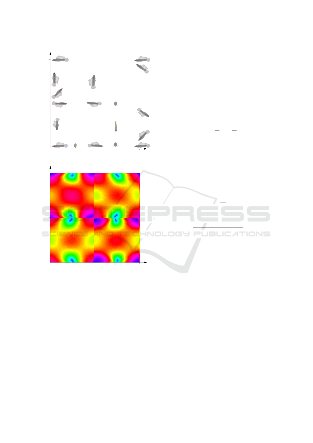
The following method is applied to measure the
standard noise deviation. Since the used pose space
depends on two parameters (pitch and yaw angle),
every feature f
n
is plotted to the 2-dimensional pa-
rameter space. In figure 1 a fish model is used to
demonstrate the 2D-pose space. The result matrix
M
f
n
is smoothed with the help of a normalized boxfil-
ter and results in
˜
M
f
n
. The standard deviation of the
n-feature’s noise σ
f
n
is calculated as following. e and
f describes the number of steps along the x- and y-
axis of the plotted feature and h = e × f the size of
the training set. f
n
8,15
for example means the value
of feature f
n
when the object is rotated 8 × s around
pitch-axis and 15 × s around yaw-axis. s is the rota-
tion angle step size in degree:
N
f
n
= M
f
n
−
˜
M
f
n
, N
f
n
(e × f ) =





f
n
1,1
f
n
1,2
··· f
n
1, f
f
n
2,1
f
n
2,2
·· · f
n
2, f
.
.
.
.
.
.
.
.
.
.
.
.
f
n
e,1
f
n
e,2
·· · f
n
e, f





(1)
n
f
n
=
1
e f
·
e
∑
i=0
f
∑
j=0
f
n
i, j
(2)
σ
f
n
=
v
u
u
t
1
e f
·
e
∑
i=0
f
∑
j=0
( f
n
i, j
− n
f
n
)
2
(3)
The feature spaces are normalized with help of σ
f
n
and the value range is shifted to zero
ˆ
f
n
e, f
=
( f
n
e, f
− min( f
n
))
σ
f
n
. (4)
Optimal Feature-set Selection Controlled by Pose-space Location
201

pitch-rotation (degree)
yaw-rotation (degree)
180
360
360180
0
x-value of 2nd quad centroid
pitch-rotation (degree)
yaw-rotation (degree)
180
360
360180
0
Fish rotation
...
...
Figure 1: Overview of the pose space (top). Normalized
feature vector (x-value of centroid) visualized along pitch
and yaw rotation of the object (bottom).
The normalized values are stored in vector
ˆ
f
n
ˆ
f
n
=





ˆ
f
n
0,0
ˆ
f
n
0,1
.
.
.
ˆ
f
n
e, f





=





ˆ
f
n
0
ˆ
f
n
1
.
.
.
ˆ
f
n
h





(5)
and brings the final normalized feature matrix
ˆ
F.
ˆ
F(h × n) =





ˆ
f
1
1
ˆ
f
2
1
·· ·
ˆ
f
n
1
ˆ
f
1
2
ˆ
f
2
2
·· ·
ˆ
f
n
2
.
.
.
.
.
.
.
.
.
.
.
.
ˆ
f
1
h
ˆ
f
2
h
·· ·
ˆ
f
n
h





(6)
After normalisation noisy features with little in-
formation have a small value range.
3.2 Feature’s Entropy
The presented method is based on the feature’s en-
tropy in relation to the 2D-parameter space. At first
a histogram with k different bins b
n
k
is calculated out
of the normalized feature vector
ˆ
f
n
, which has j
n
ele-
ments. Every bin b
n
k
has l
n
i
elements. In a next step
the entropy is calculated with
p
n
=
k
∑
i=0
l
n
i
j
n
log
2
(
l
n
i
j
n
). (7)
The number of bins k is defined for each feature
individually. Features with high information and less
noise have a high number and noisy, weak features a
little number of bins. Its number is calculated consid-
ering the normalized feature’s value range. A manu-
ally chosen constant c (e.g. 100 bins) defines the bin
number for the feature with the widest feature range.
By increasing c the number of subsets raises and the
number of pose configurations per bin falls. c should
be chosen considering the size of training set. In the
shown example c is around
1
300
of the size of the train-
ing set. The bin size |b| for all features is defined as
following:
|b| =
max(max(
ˆ
f
i
) − min(
ˆ
f
i
))
c
with
ˆ
f
i
∈
ˆ
F =

ˆ
f
0
ˆ
f
1
. . .
ˆ
f
n

.
(8)
Finally k is calculated by
k
i
= d
max(
ˆ
f
i
) − min(
ˆ
f
i
)
|b|
e
with
ˆ
f
i
∈
˜
F =

ˆ
f
0
ˆ
f
1
. . .
ˆ
f
n

.
(9)
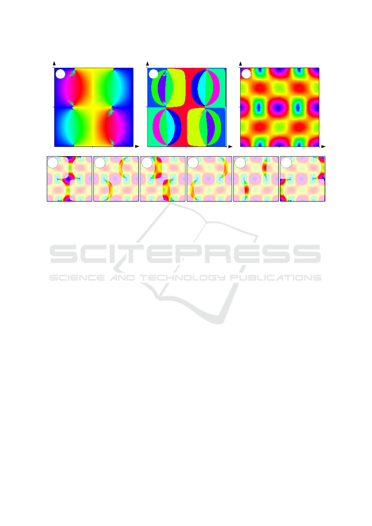
3.3 Definition and Entropy Calculation
of Feature Subsets
In a preprocessing step feature subsets for the whole
configuration space are defined. At the beginning of
the selection process the feature with the highest en-
tropy is searched:
ˆ
f
p
= max(p
i
) with i ∈ (0, 1 . . . n) (10)
Every bin b
p
k
of
ˆ
f
p
contains a set of pose config-
urations C
p
k
. Vice versa all pose configurations C
p
k
which have a similar value for feature
ˆ
f
p
are combine
in bin b
p
k
. An example is shown in figure 2 b). Each
color defines a bin b
p
k
of
ˆ
f
p
drawn over the pose con-
figuration space. In the next step all configurations
VISAPP 2016 - International Conference on Computer Vision Theory and Applications
202

a
d
e f g h
i
pitch-rotation (degree)
yaw-rotation (degree)
180
360
360180
0
b
pitch-rotation (degree)
yaw-rotation (degree)
180
360
360180
0
c
pitch-rotation (degree)
yaw-rotation (degree)
180
360
360180
0
Figure 2: Process of local entropy calculation: (a) angle of major segment axis (here feature 1) (b) feature 1 is segmented
by bins; segments are marked by different colors (c) deviation of feature 2 (d)-(i) bins of feature 1 are used to segment local
regions of feature 2. The entropy of the segmented area is calculated.
C
p
k
get an own feature matrix
˜
F
c
. This matrix includes
all features besides
ˆ
f
p
in the range of C
p
k
. An exam-
ple is shown in figure 2 d)-i). Each figure d)-i) marks
the values of a sample feature in the range of C
p
k
. Fi-
nally the feature matrices
˜
F
c
get sorted by the entropy
of each included feature vector f
k
n
(see (7)).
˜
F
c
=

f
c
0
f
c
1
. . . f
c
r

with c ∈ (0, 1 . . . k
p
) and p( f
k
0
) > p( f
k
1
)
(11)
In order to define feature subsets
˜
F
k
the number of
features per subset s ∈ (0, 1...n − 1) has to be defined
manually. The higher s is, the higher is the computa-
tional power. The number of subsets k
p
is equal to the
number of
ˆ
f
p
-bins.
˜
F
k
=

f
c
0
f
c
1
. . . f
c
s

(12)
3.4 Searching for the Right Feature
Subset
After defining subset matrices
˜
F
k
in 3.3, the right sub-
set has to be found. Therefore the feature with the
highest entropy
ˆ
f
p
has to be calculated out of the
query image. The subset
˜
F
d
is selected by sorting the
result feature value d in the right bin b
p
k
.
˜
F
d
=
˜
F
k
i f d ∈ b
p
k
(13)
4 EXPERIMENT
For a test a training set of 32400 artificial fish images
showing fish rotated around the pitch- and yaw-axis,
were used. The fish model was created in a project
described in (M
¨
uller et al., 2014). Each image has a
size of 500 x 400 pixels. A test set of 1000 images,
showing randomly rotated fish, was applied in order
to find the nearest neighbour within the 32400 images
of the training set. Simple self defined texture and
shape-based features (see 4.1) were chosen in order
to make this experiment easy to understand.
4.1 Features
For the test several simple texture- and silhouette-
based features were selected. These are shown in fig-
ure 3. In total 21 feature values were generated. A
short description of the features is given in the fol-
lowing subsections.
4.1.1 Angle of Major Segment Axis
With the help of the image moments the angle of the
silhouette’s main component is calculated. After seg-
menting the silhouette the second image moment of
the segment is calculated and is used to compute the
orientation angle α of the major segment axis (see fig-
ure 3(a)).
Optimal Feature-set Selection Controlled by Pose-space Location
203

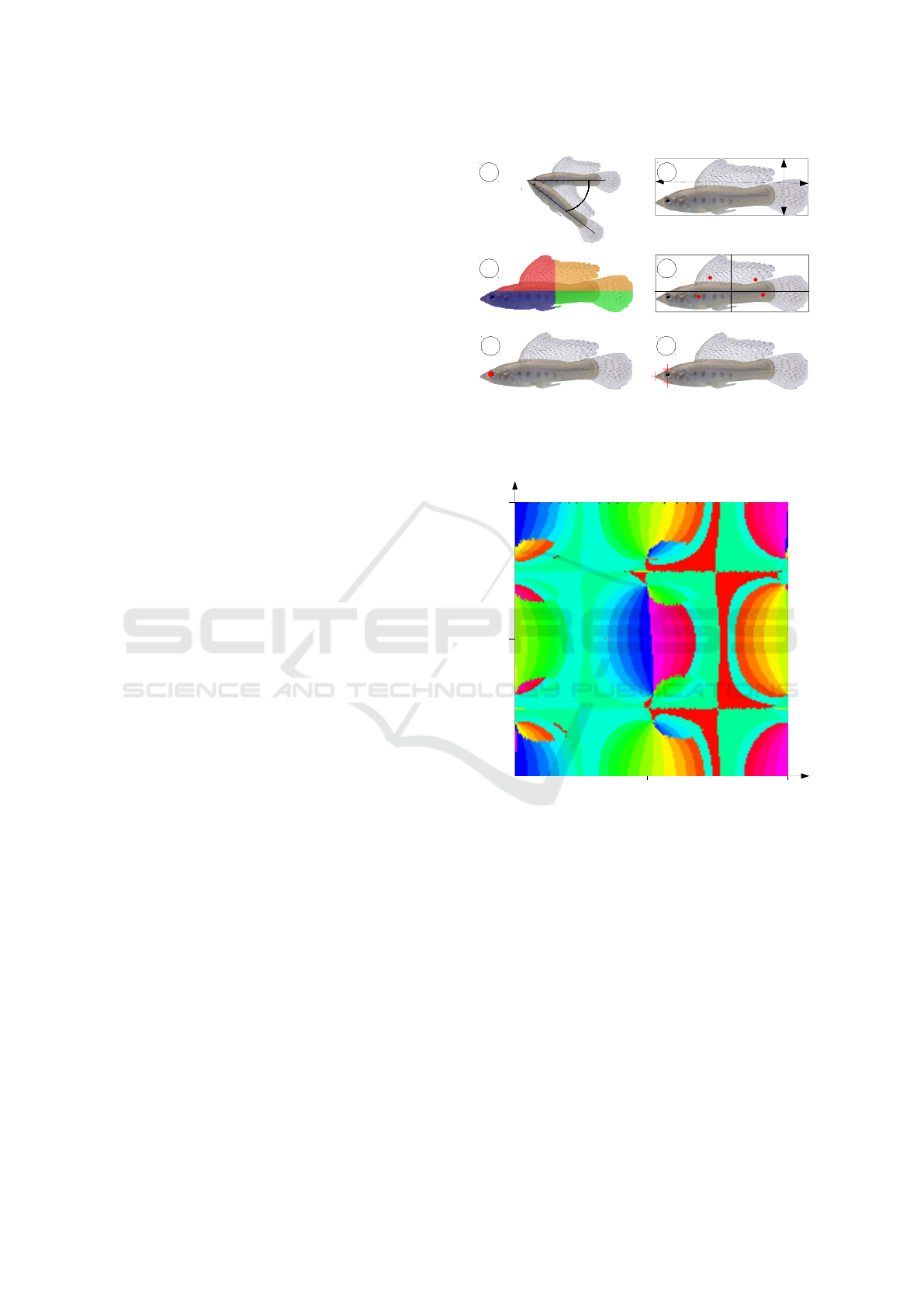
4.1.2 Ratio of Width and Height
After rotating the segment around α the segment ex-
pansion in x- and y-direction is measured. The ra-
tio between the lengths is used as feature (see figure
3(b)).
4.1.3 Centroids of Quadrants
As shown in 3(c)) the centroid of the segment’s quad-
rants is used as another feature. At first the centroid
of the rotated segment is calculated. This is used to
separate the image in four quadrants: the quadrants
are cut through the centroid parallel to x- and y-axis.
Afterwards the centroid of each quadrant is calculated
with the help of the image moments. The centroid’s
position is stored in reference to segment’s centroid.
4.1.4 Size of Quadrants
Figure 3(d) shows the feature ’size of quadrants’. The
area of every segment quadrant is calculated. In the
figure each area has another color.
4.1.5 Position of Eye
With the help of a blob detector the eye of the sam-
ple fish is searched. The exact coordinate is finally
defined by the centroid of the eye’s area.
4.1.6 Snout and Positions around Eye
The last features describe the position of the snout
(x, y) and the contour position above and below the
eye’s center. The points above and below the eye’s
center are defined by the intersection point of orthog-
onal of the major segment axis and the segment con-
tour. All coordinates are stored in relation to the seg-
ment’s centroid.
4.2 Implementation
The test application was implemented in C++ and ran
on an Intel i-7 cpu with 3.4 Ghz. For the test all fea-
tures of the training set were generated and stored in
a vector. The feature with the highest entropy (’angle
of major segment axis’) was chosen as initial feature
and 100 feature subset ranges were calculated regard-
ing 3.3. Afterwards all 1000 test images were tested
with subsets of size 5, 10, 15 and 20 and without sub-
sets. Therefore the features’ angle of major segment
axis’ was computed and the right subset was chosen
by this feature value. With the help of a brute force al-
gorithm the best fit training feature was searched. The
α
a
b
a/b
(x
1
/y
1
) (x
2
/y
2
)
(x
3
/y
3
)
(x
4
/y
4
)
(x/y)
(x
1
/y
1
)
(x
3
/y
3
)
(x
2
/y
2
)
a b
c
|a| |b|
|c| |d|
f
d
e
Figure 3: Features: (a) angle of major segment axis (b) ratio
width - height (c) centroid of quarters (d) size of quarters
(e) position of eye (f) position of snout contour pixel above
and below eye.
pitch-rotation (degree)
yaw-rotation (degree)
180
360
360180
0
subset distribution of 22 subsets (5 features per subset)
Figure 4: Distribution of subsets mapped to the pose space.
Every color shows another subset.
quality of the match was defined by the rotational er-
ror between the test and the training image of a match.
The runtime of feature extraction and matching was
measured separately.
4.3 Results
Besides the matching results the runtime of the
matching process as well as the runtime of feature ex-
traction is analysed in this section.
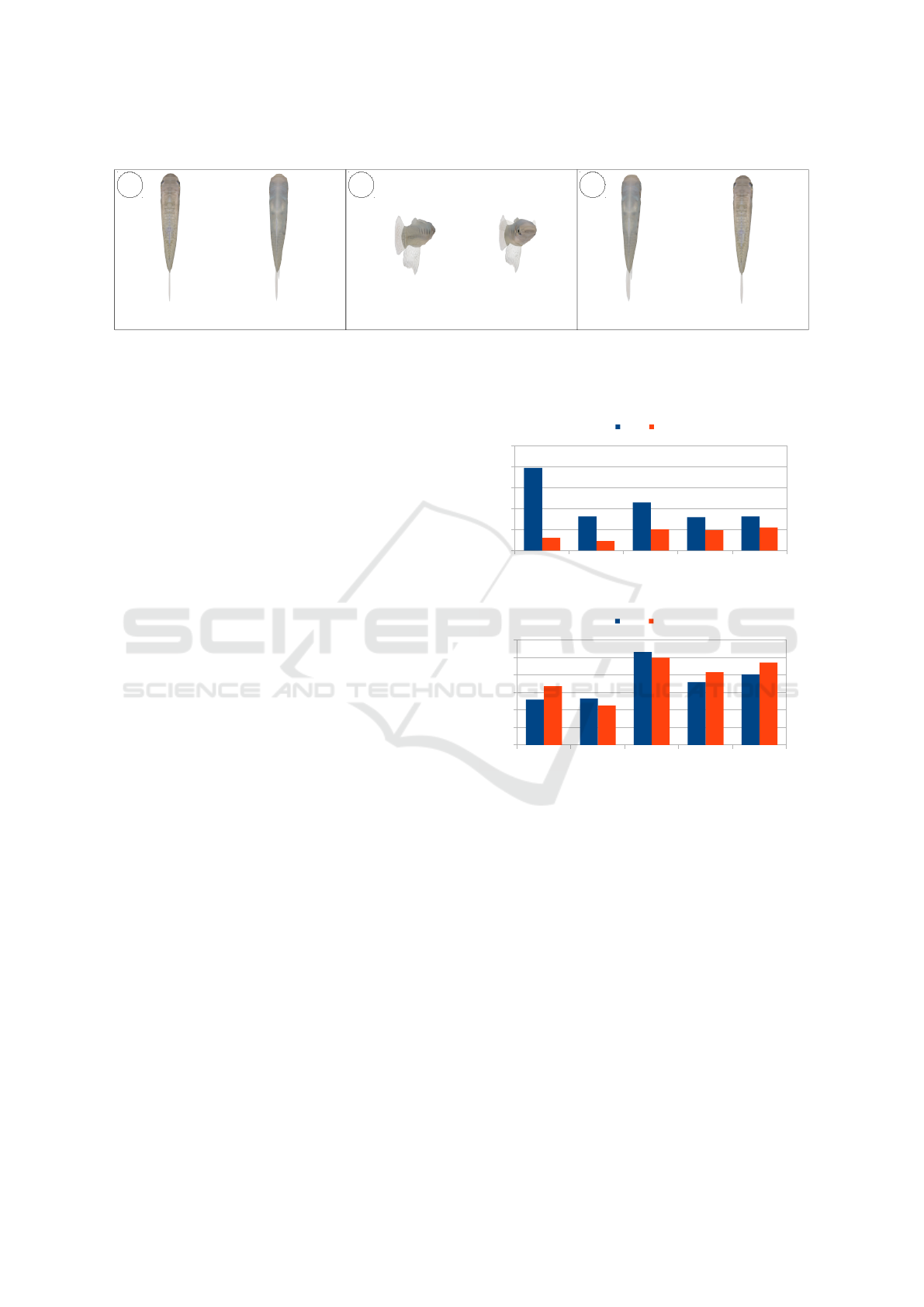
4.3.1 Pose Matching
As described in 4.2 in a first step 100 feature subset
ranges were defined. Since different subset ranges can
VISAPP 2016 - International Conference on Computer Vision Theory and Applications
204

94°/274°
92,3°/276,8°
78°/176°
203,7°/6,8°
274°/252°
275,4°/251,7°
a b c
Figure 5: Outliers: some matches affect the result negatively. The images show some outliers, causing errors around 180
degrees. On the left side the training images and on the right side the test images are shown. The rotation angle of each
images is found below (pitch-angle/yaw-angle).
include subsets with same features, the number of dif-
ferent subsets was smaller than 100. For subsets with
5 features the algorithm defines 22 different subsets
(see figure 4), for 10 features 18 different subsets, for
15 features 21 different subsets and for 20 just 1 sub-
set. This is caused by the fact, that 4 of the features
have the worst entropy in all subset ranges and are
never used. The quality of matching was measured
by calculating the pose angle difference between test-
and training image. The mean value of all angle
differences was used to measure the quality of each
method. Due to the fact that our training-database
covers just rotations in 2-degree-steps, the expected
mean error is 0.5 degrees. In general the mean-error-
value of all methods was effected negatively by some
outliers. Some of them are shown in figure 5. Since
the fish in our test is very similar from top and bottom
view, in some cases the process matched fish, which
were rotated around 180 degrees. In order to reduce
the influence of outliers in a second run the five near-
est neighbours were searched and the best match was
used to calculate the mean value. This is shown in
figure 6.
4.3.2 Runtime
The shown method can save runtime in two different
stages of the process. On the one hand it saves time
during feature extraction. It is not necessary to extract
all features out of the images, but only the features
which are part of the chosen subset. The total run-
time of the extraction process depends on the number
of features per subset. On the other hand it helps to
save runtime during the matching process. Depending
on the matching technique the time reduction is more
or less efficient, but in general matching algorithms
are faster with less features. In the shown example a
simple brute-force matching method was used. The
runtime of different configuration was measured. At
the top of figure 7 the runtime per query is shown.
The brute-force-matcher needed up to 41% less run-
5 features/subset
10 features/subset
15 features/subset
20 features/subset
all 24 features without subset
0
5
10
15
20
25
mean rotation error
Y-axis Z-axis
mean rotation-error (in degrees)
5 features/subset
10 features/subset
15 features/subset
20 features/subset
all 24 features without subset
0
0,5
1
1,5
2
2,5
3
mean rotation error (best of five)
Y-axis Z-axis
mean rotation-error (in degrees)
Figure 6: Mean matching error of all matches (top) and
mean matching error of the best out of the five nearest
neighbours (bottom).
time with a small subset than with all features. At
the bottom of the figure the time for feature extrac-
tion is shown. Due to the fact that some of the used
features depend on each other (see 4.1), in some con-
figurations all features were calculated while not all
of them was used. In spite of everything the runtime
of feature extraction was reduced by more than 50%
for subsets with 10 features and less.
5 CONCLUSION
In this work a novel approach for pose-depending
subset feature selection is proposed. In contrast to the
most other feature-based methods this method aims to
Optimal Feature-set Selection Controlled by Pose-space Location
205

5 features/subset
10 features/subset
15 features/subset
20 features/subset
all 24 features without subset
0
50
100
150
200
250
300
350
400
runtime per query (in µs)
µs
5 features/subset
10 features/subset
15 features/subset
20 features/subset
all 24 features without subset
0
2000
4000
6000
8000
10000
12000
feature extraction of 1000 samples
ms
Figure 7: (Top) Runtime of a single matching query ordered
by the number of features per subset. (Bottom) Runtime of
feature extraction process with 1000 test images.
select pose-sensitive, significant local subsets, which
fit optimal to the depending pose-space region. In a
simple experiment it could be shown, that the method
decrease the runtime of feature extraction up to 50%
and of the matching process up to 41%. Depending
on the number of features and matching-method ef-
ficiency can even be improved. During this test-run
the accuracy of the pose matching was increased as
well, in case the number of features per subset was
not chosen to small. For future it is planned to ap-
ply this method to a fish tracking system with multi-
ple degree-of-freedom fish models and contour- and
keypoint-based features.
ACKNOWLEDGEMENTS
The presented work was developed within the scope
of the interdisciplinary, DFG-funded project virtual
fish of the Institute of Real Time Learning Systems
(EZLS) and the Department of Biology and Didactics
at the University of Siegen.
REFERENCES
Amanatiadis, A., Kaburlasos, V. G., Gasteratos, A., and Pa-
padakis, S. E. (2011). Evaluation of shape descriptors
for shape-based image retrieval. Image Processing,
IET, 5(5):493–499.
Chen, C., Yang, Y., Nie, F., and Odobez, J.-M. (2011). 3d
human pose recovery from image by efficient visual
feature selection. Computer Vision and Image Under-
standing, 115(3):290–299.
Chen, C., Zhuang, Y., and Xiao, J. (2010). Silhouette rep-
resentation and matching for 3d pose discrimination–
a comparative study. Image and Vision Computing,
28(4):654–667.
Chen, C., Zhuang, Y., Xiao, J., and Wu, F. (2008). Adaptive
and compact shape descriptor by progressive feature
combination and selection with boosting. In Computer
Vision and Pattern Recognition, 2008. CVPR 2008.
IEEE Conference on, pages 1–8. IEEE.
Choi, C., Christensen, H., et al. (2010). Real-time 3d
model-based tracking using edge and keypoint fea-
tures for robotic manipulation. In Robotics and Au-
tomation (ICRA), 2010 IEEE International Confer-
ence on, pages 4048–4055. IEEE.
Collet, A., Martinez, M., and Srinivasa, S. S. (2011). The
moped framework: Object recognition and pose esti-
mation for manipulation. The International Journal of
Robotics Research, page 0278364911401765.
Hinterstoisser, S., Benhimane, S., and Navab, N. (2007).
N3m: Natural 3d markers for real-time object detec-
tion and pose estimation. In Computer Vision, 2007.
ICCV 2007. IEEE 11th International Conference on,
pages 1–7. IEEE.
Kazmi, I. K., You, L., and Zhang, J. J. (2013). A survey of
2d and 3d shape descriptors. In Computer Graphics,
Imaging and Visualization (CGIV), 2013 10th Inter-
national Conference, pages 1–10. IEEE.
M
¨
uller, K., Schlemper, J., Kuhnert, L., and Kuhnert, K.-
D. (2014). Calibration and 3d ground truth data gen-
eration with orthogonal camera-setup and refraction
compensation for aquaria in real-time. In VISAPP (3),
pages 626–634.
Payet, N. and Todorovic, S. (2011). From contours to 3d
object detection and pose estimation. In Computer Vi-
sion (ICCV), 2011 IEEE International Conference on,
pages 983–990. IEEE.
Pons-Moll, G. and Rosenhahn, B. (2011). Model-based
pose estimation. In Visual analysis of humans, pages
139–170. Springer.
Poppe, R. and Poel, M. (2006). Comparison of silhou-
ette shape descriptors for example-based human pose
recovery. In Automatic Face and Gesture Recogni-
tion, 2006. FGR 2006. 7th International Conference
on, pages 541–546. IEEE.
Rasines, I., Remazeilles, A., and Iriondo Bengoa, P. M.
(2014). Feature selection for hand pose recognition
in human-robot object exchange scenario. In Emerg-
ing Technology and Factory Automation (ETFA), 2014
IEEE, pages 1–8. IEEE.
Reinbacher, C., Ruether, M., and Bischof, H. (2010).
Pose estimation of known objects by efficient silhou-
ette matching. In Pattern Recognition (ICPR), 2010
20th International Conference on, pages 1080–1083.
IEEE.
VISAPP 2016 - International Conference on Computer Vision Theory and Applications
206

Rosenhahn, B., Brox, T., Cremers, D., and Seidel, H.-P.
(2006). A comparison of shape matching methods for
contour based pose estimation. In Combinatorial Im-
age Analysis, pages 263–276. Springer.
Optimal Feature-set Selection Controlled by Pose-space Location
207