
Probability-based Scoring for Normality Map in Brain MRI Images from
Normal Control Population
Thach-Thao Duong
LaBRI, University of Bordeaux
351 cours de la Liberation 33400 Talence, France
Keywords:
Alzheimer, Normality Map, Classification, Sparse-based.
Abstract:
The increasing availability of MRI brain data opens up a research direction for abnormality detection which
is necessary to on-time detection of impairment and performing early diagnosis. The paper proposes scores
based on z-score transformation and kernel density estimation (KDE) which are respectively Gaussian-based
assumption and nonparametric modeling to detect the abnormality in MRI brain images. The methodolo-
gies are applied on gray-matter-based score of Voxel-base Morphometry (VBM) and sparse-based score of
Sparse-based Morphometry (SBM). The experiments on well-designed normal control (CN) and Alzheimer
disease (AD) subsets extracted from MRI data set of Alzheimer’s Disease Neuroimaging Initiative (ADNI)
are conducted with threshold-based classification. The analysis of abnormality percentage of AD and CN
population is carried out to validate the robustness of the proposed scores. The further cross validation on
Linear discriminant analysis (LDA) and Support vector machine (SVM) classification between AD and CN
show significant accuracy rate, revealing the potential of statistical modeling to measure abnormality from a
population of normal subjects.
1 INTRODUCTION
The abnormality detection for brain imaging has been
emerged as an attractive research field in which the
aim is to identify the areas of impairment or abnor-
mality in the brain structure. The automatic mea-
surement of abnormality can be served as a reference
for doctors to accurately diagnose various patholog-
ical diseases. In detection of impairment in brain
structure, the difficulty increases from detecting tu-
mors, multiple sclerosis (MS), Alzheimer disease. In
detection of impairment in brain structure, detecting
multiple sclerosis (MS) is more difficult than detect-
ing tumors. Moreover, the abnormality detection of
Alzheimer disease is more difficult than both tumor
and MS because the impairments in Alzheimer ap-
pear at small or tiny areas of the brain. Impairment in
tumor shows in largest areas while multiple sclerosis
appears at several average sized locations in the brain.
Over the recent years, various automatic methods
for abnormality detection have been proposed. While
there are methods to learning the abnormality via nor-
mal and varied impairment subjects, there is still lack
of methods to measure the general abnormality solely
from the normal subjects. Among them, dictionary
learning and sparse coding is currently common in
tackling in multiple sclerosis (MS) (Deshpande et al.,
2015) and brain tumors (Irimia et al., 2012). In an-
other work, the dictionary learn from healthy brain
image tissue and sparse coding are used to automati-
cally segment multiple sclerosis (MS) lesion via un-
supervised method (Weiss et al., 2013). Having the
assumption that image patches of higher reconstruc-
tion errors contain lesions, a thresholding scheme on
the errors is used for segmentation of MS lesions.
As one of the most popular method for auto-
matic analysis of brain structure (Ashburner and Fris-
ton, 2000), VBM has been successfully applied in
the research of disorder (Radua and Mataix-Cols,
2009), aging (Huttona et al., 2009) and gender dif-
ferences (Gooda et al., 2001). While it lacks local
brain anatomy representation, patch-based approach
is efficient to capture local anatomical pattern and
inter-subjects variability. The patch-based methods
have achieved potential results in some applications
of MRI image analysis.
The main goal of this work is to to measure nor-
mality pattern at voxel level from solely normal con-
trol subjects. Recently, there is a similar work propos-
ing z-score transformation to compute abnormality
via population of normal subjects in a case study of
the children brain (Wilke et al., 2014). This work is
based on VBM methodology, where z-score is calcu-
lated from distribution of Gray Matter (GM), White
256
Duong, T-T.
Probability-based Scoring for Normality Map in Brain MRI Images from Normal Control Population.
DOI: 10.5220/0005724702540261
In Proceedings of the 11th Joint Conference on Computer Vision, Imaging and Computer Graphics Theory and Applications (VISIGRAPP 2016) - Volume 3: VISAPP, pages 256-263
ISBN: 978-989-758-175-5
Copyright
c
2016 by SCITEPRESS – Science and Technology Publications, Lda. All rights reserved

Matter (WM) and Cerebrospinal Fluid (CSF). A low-
rank and sparse components is used to exploit popula-
tion information and to identify inconsistent parts of
an image from the population which are more likely
lesions (Liu et al., 2014). However, these methods do
not construct an abnormality score at voxel level.
This work constructs a methodology to investigate
and to analyse the normality score generated from
VBM and patch-based methodology. To validate the
score, the classification is conducted on AD and CN
subjects from Alzheimer’s Disease Neuroimaing Ini-
tiative (ADNI) database. The contributions of this
work are : (i) parametric and nonparametric statistical
models at voxel level are presented to score abnormal-
ity from a training population of normal control sub-
jects, (ii) the abnormality scoring is conducted from
VBM and SBM methodologies, and (iii) the scores
are validated by the classification of AD and CN sub-
jects from ADNI database. The threshold-based is
used to validate the discrimination between AD and
CN scores while cross validation of LDA and SVM
is conducted to validate the robustness of the scores
with SVM and LDA classifiers.
2 SPARSE-BASED
MORPHOMETRY
The Sparse-Based Morphometry (SBM) is the
methodology based on the patch-based representation
(Mairal et al., 2009) at each voxel level. The patch-
based dictionary is constructed and patch-based re-
construction error is calculated from the dictionary.
This paper calls the patch-based reconstruction errors
the sparse code. The dictionary is constructed sep-
arately for each voxel from sparse code of normal
anatomical patterns. At each voxel, after being ex-
tracted and centered by subtraction of its means, a 3D
patch is normalised by dividing its norm and is vec-
torised into a vector x
i
. The dictionary of each voxel v
is constructed as a collection of N patches where N is
the size of dictionary set D . Function (1) determines
the level of sparsity where γ is a positive parameter.
The SPAMS toolbox (Mairal et al., 2009)
1
is used
to solve optimization in Function (1). Each column
of dictionary D is a vectorization of a patch encoding
the possible local morphological configurations of the
brain in the reference group D. The approximation
Dα
i
is calculated to guarantee its best closeness to the
patch x
i
via the term
1
2
kx
i
− Dα
i
k
2
2
k. The purpose of
the term kα
i
k is to ensure that each extracted patch x
i
is able to be decomposed in a sparse way in the output
1
http://spams-devel.gforge.inria.fr/index.html
dictionary D.
F = min
D,α
i
|D|
∑
i=1
1
2
kx
i
− Dα
i
k
2
2
+ γkα
i
k
1
(1)
At a voxel v of an input subject Q, a patch p
v
Q
is processed identically to the dictionary construc-
tion. Via the reconstruction mapping, the sparse-
based score SM is the reconstruction cost to retrieve
the closed relevant patch matched from the dictionary
at the corresponding location.
SM
v
Q
= f (p
v
Q
, v) = min
α∈R
p
1
2
kp
v
Q
−D
v
αk
2
2
+γkαk
1
(2)
D
v
is the dictionary associated with the voxel at
location v. The dictionary D is expected to have the
capacity to sparsely reconstruct majority of the nor-
mal patches learned in D. Therefore, giving an abnor-
mal brain subject such as AD, an approximation error
1
2
kx − D
v
αk
2
2
would converge to a low sparity level,
resulting statistical high values of kαk
1
and SM
v
Q
. Ac-
cordingly, the value of function f is relatively high for
abnormal brain anatomy voxel and relatively low for
normal voxel.
3 NORMALITY SCORING
This paper employs a subpart of the standardised
ADNI1 collection (Wyman et al., 2013) which is
a commonly used dataset in Alzheimer disease re-
search. Two groups of cognitively normal subjects
(CN), named “CN Dictionary” and “CN Training”,
are constructed for dictionary and for mapping upon
normal population. The CN dictionary is a collection
of sparse representation of normal brain anatomy. The
CN Training is a population representing for normal
brain anatomy on which an unknown-pathology sub-
ject is projected for its normality measurement. In
addition, two groups of CN and AD subjects are ex-
tracted for testing. To minimise bias of the experi-
ments, these four groups are randomly selected with
the same size of 70 subjects and similar correlation in
age and gender distribution.
Figure (1) shows the SBM and VBM methodolo-
gies to generate the abnormality map. The final goal
of both methodologies is to measure the abnormality
at voxel level, leading to an abnormality map. SBM
methodology requires a Dictionary of patches con-
structed at each voxel to measure the sparse-based re-
construction cost SM. The SM values of an input sub-
ject are projected on the distribution of training CN
subjects to measure the abnormality at the associated
voxel location. This procedure is repeated with gray
Probability-based Scoring for Normality Map in Brain MRI Images from Normal Control Population
257
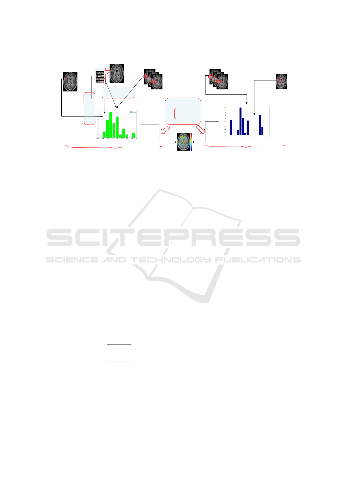
Training subjects
x
Distribution of SM from training CN
Input subject
Dictionary
Abnormality Map
Distribution of GM from training CN
x
Transformation
Sparse-based framework Vorxel-based framework
z-score
KDE
Input subject
Training subjects
R
e
c
o
n
s
t
r
u
c
t
i
o
n
C
o
s
t
Reconstruction
Cost
Figure 1: An overview diagram of the methods.
matter GM value in VBM methodology. The projec-
tion of a single value over a distribution is performed
via z-score and KDE estimation.
3.1 Z-score
The abnormality score is calculated from the projec-
tion upon the training set T . In VBM methodology,
for each voxel, assuming that the distribution of GM
value of T as Gaussian distribution, z-score transfor-
mation is employed to scale it to the standard Gaus-
sian distribution so that the abnormality score is mea-
sured upon the same standard normal distribution. For
the input subject S, the zGM score is computed ac-
cording to the Functions (3) and (5). GM score of the
subjects Q at voxel v is denoted as GM
v
Q
. The zGM
v
S|T
is the GM score at voxel v of the subject Q projected
on the normal population T . The score zGM of the
subjects S is the average of zGM
v
. The µ
v
T
and σ
v
T
are mean and standard deviation of the distribution of
GM values of subjects in T at the particular voxel v,
denoted as {GM
v
|T }.
zGM
v
S|T
=
GM
v
S
− µ
v
T
σ
v
T
(3)
zSM
v
S|T
=
SM
v
S
− µ
v
T
σ
v
T
(4)
zGM
S|T
= avg
v
{zGM
v
S|T
} (5)
zSM
S|T
= avg
v
{zSM
v
S|T
} (6)
Similarly in SBM methodology, the zSM is calcu-
lated with the Functions (4) and (6). µ
v
T
and σ
v
T
are
the mean and the standard deviation of the distribution
{SM
v
|T }. zSM
S|T
denotes the score transformed by
z-score over the distribution of the normal population
T .
3.2 Kernel Density Estimation (KDE)
The normality measurement can be addressed by the
statistical principle of anomaly detection which is
stated that “an abnormality is an observation which is
suspected of being partially or wholly irrelevant be-
cause it is not generated by the stochastic model as-
sumed” (Anscombe and Guttman, 1960). To avoid
biased assumption of the underlying distribution of
the stochastic model, kernel density estimation (KDE)
(Rosenblatt, 1956; Parzen, 1962) which is a nonpara-
metric technique to estimate the density probability
distribution and to measure the probability of x be-
longing to the distribution X. This probability P(x, X )
for x to belong to the distribution X is calculated by
the default KDE function in MATLAB.
Given an input GM
v
S
, the probability of that voxel
to be normal is the probability of that voxel belonging
to the distribution computed according to the Func-
tions (7) and (9). The normality score of the sub-
ject S is calculated as the average of the score kGM
v
.
kGM
S|T
denotes the score transformed by KDE over
the distribution of normal population T .
kGM
v
S|T
= P(GM
v
S
|{GM
v
|T }) (7)
kSM
v
S|T
= P(S M
v
S
|{SM
v
|T }) (8)
kGM
S|T
= avg
v
{kGM
v
S|T
} (9)
kSM
S|T
= avg
v
{kGM
v
S|T
} (10)
Similar to the score kGM, the sparse-based nor-
mality score by KDE is also computed by the Func-
VISAPP 2016 - International Conference on Computer Vision Theory and Applications
258

tions (8) and (10). kGM
S|T
denotes the score trans-
formed by KDE over the distribution of normal pop-
ulation T .
4 EXPERIMENTS
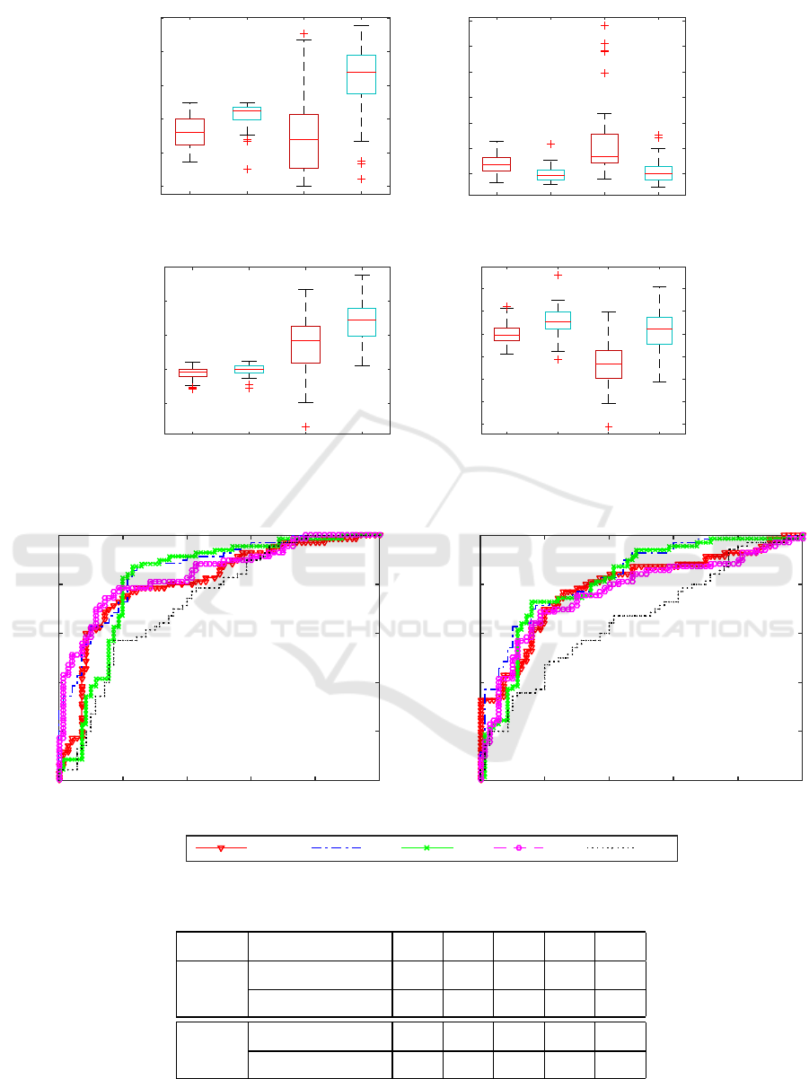
To validate the robustness of proposed scores in mea-
suring the normality at voxel level, the evaluation of
the distinction on Alzheimer patients is performed
four scores and volume calculated within whole brain
and hippocampus since impairment in hippocampus
is the most contributing factor for AD disease (Braak
and Braak, 1991). Because of high complexity in
sparse-based reconstruction from dictionary learning,
the MRI image resolution is scaled down to half of
the original dimension. In addition, in order to reduce
time and resource to process voxels with low conver-
gence of GM, only voxels with the GM higher than
the threshold ε = 0.1 are processed. volume is calcu-
lated as the total number of voxels.
Vol
S
=
∑
v
(GM
v
S
≥ ε) (11)
The Figure (2) provides a comparison between
proposed scores calculated on testing AD and test-
ing CN subjects. The scores kSM, kGM and zGM
measure the normality while the score zSM measure
the abnormality because high SM presents large re-
construction cost from the dictionary and high GM
indicates the high convergence of gray matter. The
figure reveals that normality score in hippo campus
has wider range than that of the whole brain. More-
over, hippocampus has experienced a more significant
difference between AD and CN scores than the whole
brain. This statistically significant difference is shown
by the t-test where p ≤ 10
−5
, except the case of kGM
in the whole brain with p = 0.0012.
4.1 Threshold-based Classification
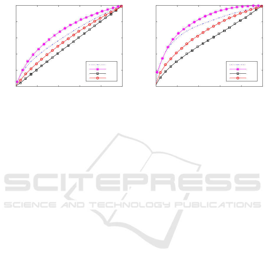
The Figure (3) presents the ROC curve of threshold-
based classification between AD and CN by volume
and proposed scores. The Table (2) lists the area un-
der the cure (AUC) and the cut-point for each classi-
fication. It is clearly from the Figure (3) that the clas-
sification on hippocampus are generally better than
that on whole brain. In addition, the AUC and cut-
point for hippocampus are generally higher than that
of whole brain. In term of AUC, the zSM achieves the
best performance while kSM gains the best accuracy
at cut-point. Seen from the AUC in hippocampus of
the Table (2), the score zSM, kSM and zGM achieve
the comparable AUC with more than 82% and better
than volume. Meanwhile, kGM gains the worse per-
formance among score, which is apparent because its
significance p value from t-test are the highest among
others.
The abnormality percentage in the area of obser-
vation (e.g. whole brain or hippocampus) is calculate
to evaluate the abnormality at voxel level. The ab-
normality percentage is the ratio of number of abnor-
mal voxel to the volume of the area of observation.
A voxel is identified as abnormal if its score is above
the threshold. In the observation of CN population,
the score of every voxel of 70 CN subjects is collected
and ranked. An array of thresholds is calculated based
on training population so that abnormality percentage
of ranging from 0% to 100% of abnormality of the
test CN population T . Accordingly to the array of
thresholds, the abnormality percentage are calculated
for each subjects of the AD and CN population. Plot-
ted in figure 4, abnormality percentage of AD and CN
population are the averages of abnormality percentage
over subjects within each populations.
The Figure 4 shows the correlation of abnormal-
ity percentage of AD and CN computed whole brain
and hippocampus according to the array of thresh-
olds. The y-axis presents the abnormality percentage
of AD subjects while the x-axis presents the associ-
ated abnormality percentage of CN population from
the identical thresholds. It is clear that the abnor-
mality percentage computed in whole brain is signifi-
cantly higher than that in hippocampus, which means
there are larger areas of abnormality in hippocampus
or abnormal regions in hippocampus. It is clearly
from the Fig. 4 that the kSM and zSM show better
abnormality percentage than kGM and zGM respec-
tively. In a closer look, kSM and zSM show higher
abnormality percentage than kGM and zGM, which
means the kSM and zSM show the robustness of ab-
normality measurement in AD. The kSM and zSM
show the clear distinction in terms of abnormality per-
centage among AD than kGM and zGM.
4.2 Cross-validation with LDA and
SVM
Additional validation the robustness of scores mea-
suring the normality at voxel level are conducted on
classification between AD and CN with two clas-
sifiers Linear discriminant analysis (LDA) (Fisher,
1936) and Support vector machine (SVM) (Cortes
and Vapnik, 95) via leave-one-out-cross-validation
(LOOCV) (Devijver and Kittler, 1982). The LOOCV
is employed to minimise bias.
The Table 2 presents classification rates in per-
centage of two classifiers LDA and SVM between AD
Probability-based Scoring for Normality Map in Brain MRI Images from Normal Control Population
259
AD CN AD-H CN-H
Normality
0
10
20
30
40
50
kSM
AD CN AD-H CN-H
Abnormality
0
2
4
6
8
10
12
zSM
AD CN AD-H CN-H
Normality
1.5
2
2.5
3
kGM
AD CN AD-H CN-H
Normality
-2
-1.5
-1
-0.5
0
0.5
1
zGM
Figure 2: The comparison of the (ab)normality score between AD and CN in whole brain and hippocampus region. ’AD-H’
and ’CN-H’ denote the scores calculated in hippocampus.
False positive rate
0 0.2 0.4 0.6 0.8 1
True positive rate
0
0.2
0.4
0.6
0.8
1
ROC for Classification on Hippocampus
Volume zSM kSM zGM kGM
False positive rate
0 0.2 0.4 0.6 0.8 1
True positive rate
0
0.2
0.4
0.6
0.8
1
ROC for Classification on whole brain
Figure 3: ROC curves of proposed scores for threshold-based classification between AD and CN.
Table 1: AUC and cut-point in percentage of ROC curves from Figure 3.
Area of Observation Vol zSM kSM zGM kGM
AUC whole brain 79.04 83.39 81.29 76.82 65.90
hippocampus 81.01 86.29 82.22 84.67 73.08
cut-point whole brain 77.14 74.29 74.29 71.43 60.00
hippocampus 74.29 78.57 80.00 78.57 65.71
VISAPP 2016 - International Conference on Computer Vision Theory and Applications
260
0 20 40 60 80 100
Abnormalilty Percentage of CN
0
0.2
0.4
0.6
0.8
1
Abnormalilty Percentage of AD
Whole brain
kSM
zSM
kGM
zGM
0 20 40 60 80 100
Abnormalilty Percentage of CN
0
0.2
0.4
0.6
0.8
1
Hippocampus
kSM
zSM
kGM
zGM
Figure 4: Correlation of Abnormality Percentage in whole brain and hippocampus between AD and CN.
and CN subjects based on the volume, four abnormal-
ity scores transformed from SBM and V BM method-
ology. The classification is performed on whole
brain and hippocampus areas. The hippocampus ob-
served in this work comprises four regions of inter-
est (ROI): hippocampus left, hippocampus right, para
hippocampus left, para hippocampus right, which is
defined in the Automatic Anatomical Labeling (AAL)
(Tzourio-Mazoyer et al., 2002). The classification
rates are measured in terms of accuracy, sensitivity,
specificity which are abbreviated as “Acc”, “Sen” and
“Spec” in the tables. Features for classifiers LDA and
SVM are “Vol” standing for Volume, zGM, kGM,
zSM and kSM. For convenient presentation, the ex-
pression of “classifier”-“feature” is used to mention
that classifier with the specific feature. For example,
LDA-zGM represents classifier LDA with zGM.
Seen from the table, while impairment in hip-
pocampus region is the most contributed factors for
AD disease (Braak and Braak, 1991), the volume of
hippocampus gained less improved than the volume
of the whole brain. This fact proved that the fea-
ture on volume does not reveal accurately the abnor-
mality degree of the brain. On the other hand, vol-
ume feature lacks of capability to rank or measure
the abnormality in voxel level instead the score show
the score for brain or region levels. In regard to ac-
curacy rate in whole brain, LDA-Vol, SVM-Vol and
LDA-kSM achieved the best performance at 72.86%.
Most of classifications with four scores do not im-
prove upon this classification rate but classification
procedures on hippocampus areas. Among them the
highest accuracy of classification is SVM and LDA
with kSM score on hippocampus regions, accounting
for 82.14% and 80.71% respectively. In most of the
case except the case of SVM on zGM score, the score
calculated in hippocampus areas achieved better per-
formance in term of classification rate than that calcu-
lated in the whole brain. The improvement of classi-
fication rate in hippocampus areas reveals the robust-
ness of model in measuring the abnormality score. It
is evident from the table, the z-score transformations
of GM and SM do not significantly improve the clas-
sification rate compared with volume feature both on
whole brain and hippocampus except LDA-zGM with
76.43% and SVM-zGM with 75.71%. In further anal-
ysis, to compute the robustness of the score in terms
of the classification rate between the whole brain and
hippo campus areas, the gap between whole brain and
hippocampus is calculated.
The table 3 presents the subtraction classifica-
tion rate of whole brain from hippocampus. This
subtraction is computed on accuracy, sensitivity and
specificity rate. The feature volume and SVM show
the degraded performance in terms of accuracy rate,
revealing that volume feature is not a proper fea-
ture measuring abnormality. While the SVM-kSM
achieved the best improvement in hippocampus ar-
eas(i.e. 12.14%), the one on zSM degraded perfor-
mance at a negative gap of -2.86%, proving a conclu-
sion that KDE transformation is better than z-score
transformation in computing abnormality score. In
addition, KDE is considerably better than z-score
transformation in two cases of LDA on SM and SVM
on GM (i.e. 7.86% vs 1.43 % and 10.71% vs 4.29%)
while there is a mere degradation of KDE with z-score
on LDA on GM (i.e. LDA-kGM of 5.00% vs LDA-
zGM of 5.71%).
Via KDE transformation, SM score show im-
provements over GM score for particular cases such
as with SVM classifier (i.e. SVM-kSM of 12.14%
vs SVM-kGM of 10.71%), LDA classifier (i.e. LDA-
kSM of 7.86% vs LDA-kGM of 5.00%)
Assuming in the experiments that positive and
Probability-based Scoring for Normality Map in Brain MRI Images from Normal Control Population
261
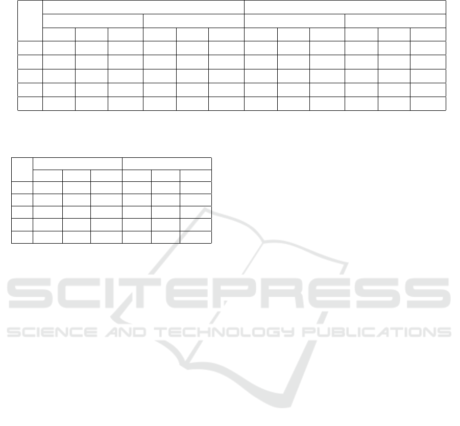
Table 2: LDA and SVM classification with score of Volume, zGM , kGM, zSM and kSM for whole brain and Hippocampus
region.
LDA SVM
Score whole brain Hippocampus whole brain Hippocampus
Acc (%) Sen (%) Spec (%) Acc (%) Sen (%) Spec (%) Acc (%) Sen (%) Spec (%) Acc (%) Sen (%) Spec (%)
Vol 72.86 78.57 67.14 70.71 80.00 61.43 72.86 78.57 67.14 66.43 82.86 50.00
zGM 70.71 68.57 72.86 76.43 75.71 77.14 71.43 65.71 77.14 75.71 75.71 75.71
kGM 60.71 65.71 55.71 65.71 77.14 54.29 53.57 71.43 35.71 64.29 90.00 38.57
SM 72.14 77.14 67.14 73.57 91.43 55.71 70.71 77.14 64.29 67.86 94.29 41.43
kSM 72.86 81.43 64.29 80.71 84.29 77.14 70.00 81.43 58.57 82.14 87.14 77.14
Table 3: Gap of classification rate between whole-brain and
hippocampus.
Score LDA SVM
Acc (%) Sen (%) Spec (%) Acc (%) Sen (%) Spec (%)
Vol -2.14 1.43 -5.71 -6.43 4.29 -17.14
zGM 5.71 7.14 4.29 4.29 10.00 -1.43
kGM 5.00 11.43 -1.43 10.71 18.57 2.86
zSM 1.43 14.29 -11.43 -2.86 17.14 -22.86
kSM 7.86 2.86 12.86 12.14 5.71 18.57
negative are denoted as CN subject and AD subjects,
it is preferable for classification methodologies with
high Specificity because of preventive cure for the dis-
ease. It is clearly from the Table 2, SVM-kSM per-
formed the best in terms of specificity, accounting for
77.14% while SVM-zGM gained the highest sensitiv-
ity rate at 94.29%. Moreover, in the Table 3, the SVM
and LDA on kSM have significant gap of specificity
rate with 18.57% and 12.86% respectively. On the
other hand, volume feature degraded the specificity
with negative gaps of -17.14% and -5.71%. There is
a drop in specificity of 22.86% and 11.43% for SVM
and LDA on zSM respectively. In the case of GM
score, the gaps of specificity are considerably small
except LDA-zGM at 4.29 %.
5 CONCLUSIONS
This paper has introduced methodologies for abnor-
mality scoring from solely projecting on normal pop-
ulation via VBM and SBM methodologies. Inspired
by the statistical anomaly detection techniques, z-
score transformation, i.e. standardised Gaussian-
based assumption, and KDE, i.e. nonparametric sta-
tistical model, are used. Since the scores are mea-
sured by only CN subjects, the methods can be effi-
ciently implemented without prior knowledge of ab-
normality. The method is applied on GM from VBM
methodology and sparse code from SBM methodol-
ogy. The sparse code is deduced from dictionary
learning and sparse representation of a separate nor-
mal population. Subsets of CN and AD popula-
tion are extracted from ADNI database with similar
cohesion of age and gender. Finally, the proposed
score is evaluated via threshold-based classification
and the robustness is demonstrated by achieving the
best AUC and cut-point rates of 86.29% and 80%, re-
spectively. Additionally, AD population has higher
abnormality percentage than CN, demonstrating the
novelty of proposed scores in measurement of nor-
mality. The results are significantly potential for fur-
ther applications to the detection of other patholo-
gies since the normality scores calculated solely from
CN patient are able to detect Alzheimer disease with
simple threshold classification. Additionally, the pro-
posed score is evaluated via SVM and LDA classi-
fiers within LOOCV procedure and the robustness is
demonstrated by gaining the accuracy and sensitivity
rates of more than 80% and 90%, respectively.
ACKNOWLEDGEMENTS
This study has been performed with financial support
from the French National Research Agency (ANR) in
the Investments for the future Programme IdEx Bor-
deaux, Cluster of excellence CPU. The dataset was
obtained from the Alzheimer’s Disease Neuroimag-
ing Initiative (ADNI). The author thanks Dr. Pierrick
Coup
´
e for sharing some parts of the dataset for this
study. Dataset providers, however, did not participate
in analysis or writing of this report.
REFERENCES
Anscombe, F. J. and Guttman, I. (1960). Rejection of out-
liers. 2(2):123–147.
Ashburner, J. and Friston, K. J. (2000). Voxel-based mor-
phometrythe methods. NeuroImage, 11(6):805–821.
VISAPP 2016 - International Conference on Computer Vision Theory and Applications
262

Braak, H. and Braak, E. (1991). Neuropathological stageing
of alzheimer-related changes. Acta Neuropathologica,
82(4):239–259.
Cortes, C. and Vapnik, V. (’95). Support-vector networks.
Mach. Learn., 20(3):273–297.
Deshpande, H., Maurel, P., and Barillot, C. (2015). Classi-
fication of Multiple Sclerosis Lesions using Adaptive
Dictionary Learning. Computerized Medical Imaging
and Graphics, pages 1–15.
Devijver, P. A. and Kittler, J. (1982). Pattern recognition:
A statistical approach. Prentice Hall.
Fisher, R. A. (1936). The use of multiple measurements in
taxonomic problems. Annals of Eugenics, 7(7):179–
188.
Gooda, C. D., Johnsrudeb, I., Ashburnera, J., Hensona,
R. N., Fristona, K. J., and Frackowiaka, R. S. (2001).
A comparison between voxel-based cortical thickness
and voxel-based morphometry in normal aging. Neu-
roImage, 14(3):685–700.
Huttona, C., Draganskia, B., Ashburnera, J., and
Weiskopfa, N. (2009). A comparison between voxel-
based cortical thickness and voxel-based morphome-
try in normal aging. NeuroImage, 48(2):371–380.
Irimia, A., Wang, B., Aylward, S. R., Prastawa, M. W.,
Pace, D. F., Gerig, G., Hovda, D. A., Kikinis, R.,
Vespa, P. M., and Horn, J. D. V. (2012). Neuroimag-
ing of structural pathology and connectomics in trau-
matic brain injury: Toward personalized outcome pre-
diction. NeuroImage: Clinical, 1(1):1 – 17.
Liu, X., Niethammer, M., Kwitt, R., McCormick, M., and
Aylward, S. R. (2014). Low-rank to the rescue - atlas-
based analyses in the presence of pathologies. In MIC-
CAI (3)’14, pages 97–104.
Mairal, J., Bach, F., Ponce, J., and Sapiro, G. (2009). Online
dictionary learning for sparse coding. In Proceedings
of the 26th ICML, pages 689–696.
Parzen, E. (1962). On estimation of a probability den-
sity function and mode. The Annals of Mathematical
Statistics, 33(3):pp. 1065–1076.
Radua, J. and Mataix-Cols, D. (2009). Voxel-wise
meta-analysis of grey matter changes in obsessive-
compulsive disorder. The British J. of Psychiatry,
195(5):393–402.
Rosenblatt, M. (1956). Remarks on Some Nonparametric
Estimates of a Density Function. The Annals of Math-
ematical Statistics, 27(3):832–837.
Tzourio-Mazoyer, N., Landeau, B., Papathanassiou, D.,
Crivello, F., Etard, O., Delcroix, N., Mazoyer, B., and
Joliot, M. (2002). Automated anatomical labeling of
activations in {SPM} using a macroscopic anatomi-
cal parcellation of the {MNI} {MRI} single-subject
brain. NeuroImage, 15(1):273 – 289.
Weiss, N., Rueckert, D., and Rao, A. (2013). Multiple
sclerosis lesion segmentation using dictionary learn-
ing and sparse coding. In Medical Image Computing
and Computer-Assisted Intervention - MICCAI, pages
735–742.
Wilke, M., Rose, D. F., Holland, S. K., and Leach, J. L.
(2014). Multidimensional morphometric 3d mri anal-
yses for detecting brain abnormalities in children: Im-
pact of control population. Human Brain Mapping,
35(7):3199–3215.
Wyman, B. T., Harvey, D. J., Crawford, K., Bernstein,
M. A., Carmichael, O., Cole, P. E., Crane, P. K., De-
Carli, C., Fox, N. C., Gunter, J. L., Hill, D., Killiany,
R. J., Pachai, C., Schwarz, A. J., Schuff, N., Senjem,
M. L., Suhy, J., Thompson, P. M., Weiner, M., and Jr.,
C. R. J. (2013). Standardization of analysis sets for
reporting results from ADNI MRI data. Alzheimer’s
& Dementia, 9(3):332 – 337.
Probability-based Scoring for Normality Map in Brain MRI Images from Normal Control Population
263
