
Low Latency Action Recognition with Depth Information
Ali Seydi Keceli
and Ahmet Burak Can
Computer Engineering Department, Hacettepe University, Ankara, Turkey
Keywords: Action Recognition, RGB-D Sensor, Adaboost, SVM, Low Latency.
Abstract: In this study an approach for low latency action recognition is proposed. Low latency action recognition
aims to recognize actions without observing the whole action sequence. In the proposed approach, a skeletal
model is obtained from depth images. Features extracted from the skeletal model are considered as time
series and histograms. To classify actions, Adaboost M1 classifier is utilized with an SVM kernel. The
trained classifiers are tested with different action observation ratios and compared with some of the studies
in the literature. The model produces promising results without observing the whole action sequence.
1 INTRODUCTION
Recognizing actions of humans is one of the
important problems in computer vision. Since an
action can be viewed from different angles and
dimensions, it is still very hard to recognize actions
with high accuracy. Furthermore, variety among
human bodies and differences among subjects while
performing the same actions increase the difficulty
of the problem. Most of the current methods in the
literature require to see the whole action sequence
for recognition and classification. Low latency
recognition is a recent and progressively growing
trend in the field of action recognition. In low
latency recognition methods, actions are classified
by seeing only a part of the sequence. Since less
information is used in these methods, classification
ratio generally drops comparing to the whole action
recognition methods. Thus, only in a few study, low
latency action recognition is studied (Ellis, 2013;
Zanfir et al., 2013).
This paper introduces a low latency action
recognition method. In this method, depth data is
used to construct a skeletal joint model. Joint
positions, position differences, distance from initial
positions, joint angles, and joint displacements are
extracted as features from this skeletal model. While
joint positions, position differences, and distance
from initial positions are evaluated as time series,
joint angles are considered as histograms. Joint
displacements are evaluated as numeric values.
These features are used by an Adaboost classifier to
recognize actions.
Adaboost classifier is trained with a Radial Basis
Function (RBF) based support vector machine
(SVM) kernel. The trained model is tested with
different observation ratios of actions. The model
produces meaningful results even 30% of an action
is observed.
The outline of the paper is as follows. Section 2
gives the related work in the literature. Section 3
introduces the proposed model. Section 4 explains
the classification phase. Section 5 gives the
experimental results. Finally in Section 6
conclusions about the results are given.
2 RELATED WORK
One of the most successful methods in the literature
is developed by Zanfir et al., (2013). This method
uses the features extracted from a skeletal model that
is proposed by Shotton et al., (2013) This skeletal
model has a wide usage in action recognition
studies. The positions of the skeletal joints and the
first and second degree derivatives of these joint
locations are used as features in this method. The
derivatives of the joint locations are calculated by
sliding a window over the action sequence. The
feature extraction step is applied on all frames one
by one. Before the feature extraction, normalization
is made on the joint locations to minimize the
differences that could occur due to varying height
and positions of the actors (subjects). The joint
position normalization algorithm is shown below. In
590
Keceli, A. and Can, A.
Low Latency Action Recognition with Depth Information.
DOI: 10.5220/0005723005900596
In Proceedings of the 11th Joint Conference on Computer Vision, Imaging and Computer Graphics Theory and Applications (VISIGRAPP 2016) - Volume 4: VISAPP, pages 590-596
ISBN: 978-989-758-175-5
Copyright
c
2016 by SCITEPRESS – Science and Technology Publications, Lda. All rights reserved

this algorithm
is the position of the root
joint,
represents the mean lenght of the limbs and
is the distance between two joints. A bread first
search is made to traverse the joints and
is the
last joint that is reached at the end.
,
←
←
←
,
||
||
,
←
,
,….
,
First relative positions of the joint location according
to hip joint are calculated. After normalization and
feature extraction stages, descriptive frame selection
is made. The purpose of the descriptive frame
selection is to find smallest descriptive subset that
represents the action sequence. To solve this
problem classification is made during training. In the
selection of a frame ratio between all neighbour
frames and the neighbour frames that belongs the
same action is calculated. If the calculated value is
greater than a defined threshold, frame is selected.
After the selection of key frames, classification is
made. KNN (Altman 1992) classifier is used as base
classifier. Classification algorithm is shown below.
In the algorithm
is the training set and
is the confidence value of the classifier.
,
←
∈
←
∑
Another method that tries to recognize actions with
low latency is proposed by Ellis et al. (Ellis 2013).
This study reaches 88.7% and 65.7% true
classification ratio with MSRC-12 (Hoai and de la
Torre, 2014) and MSR-Action 3D datasets. But
while testing the method cross-validation test is
applied instead of cross-subject test. This method
uses difference between the joint positions of a
frame and the joint positions 5 and 30 frame before.
Difference operation is made by calculating the
Euclidian distance between positions of the same
joints. Another feature set is the difference between
position of a joint and positions of the all joints 10
frame before. After extraction of the features
different models are trained. First Bag of Words
approach is applied. Frames are clustered into 1000
sets. All frames are labelled with a set label and all
action sequences are converted into a sequence of
labels. Then label histogram for all actions are
calculated. These histograms are classified with a
SVM classifier. The second model in this study uses
Conditional Random Field (CRF). The recognition is
done by seeing only first 30% of the frames of an
action. Although limited ratio of the frames are used
in recognition a high recognition ratio like %90 is
reached with cross-validation testing method.
Hoai and de la Torre (2014) proposed another
low latency action recognition method which works
for video sequences. This method recognize actions
on line. First actions are segmented. Segment is
given as an input for all action classifiers and the
label of the classifier which give the largest value is
assigned to segment. Then this process continues
with the other segments. This method used HMM,
SVM and Structured Output SVM (SOSVM) as
classifiers. The recognition is done with 30% of the
frames of an action and 65% true classification ratio
is reached.
3 LOW LATENCY ACTION
RECOGNITION
In this paper a low latency action recognition
method is introduced. This method uses features
extracted from Shotton et al.’s skeletal model
(Shotton et al., 2013). While some features extracted
from each frame are used as time series, others
extracted from the observed part of the sequence are
used as histograms and numeric values.
For the features used as time series, dimension
reduction is applied with the method referred in
(Khushaba et al., 2007). In this method, wavelet
packet transform (WPT) is applied first over the
sequence. The sequence is divided into two sub
bands. These sub signals are scale and wavelet
functions that are placed in a new vertical basis. This
process is achieved with the usage of a filter bank.
Features from the time series are obtained by
Low Latency Action Recognition with Depth Information
591

JointPositionInf ormation
DerivativeoftheJointPositions
JointDistancefromInitialPosition
JointAngleHistograms
JointDisplacements
TimeSeriesFeatureExraction
Ada Boost
SVM
Figure 1: Flow chart of Low Latency Action Recognition.
calculating the energy values of wavelet coefficients.
This calculation is shown in Equation-1. Every
subspace in WPT tree are taken as a new feature
space. For every subspace square of WPT
coefficients are summed and divided into number of
coefficients. Finally logarithm of the summation is
calculated for normalization.
,
log
∑
,,
⁄
)
(1)
,,
describes the output signal obtained by WPT
transform and 2
⁄
is the number of the
coefficients in the subband. As a result of this
process, fixed length features are constructed from
the diffferent lenght feature sequences. Thus actions
with different lengths are brought to a common
extent. However this process cause an over
dimensioning problem of the data depending on the
depth of WPT tree. The length of the output feature
vector can vary according to given input
parameter.
After obtaining all features, classification phase
is started. Adaboost ensemble classifier is used for
prediction. SVM is used as the base classifier in
boosting. Steps of the developed method are shown
in Figure-1. Extracted features that are considered as
time series and histograms are combined and then
Adaboost classifier utilized.
3.1 Features
As mentioned earlier, Shotton et al.’s joint skeleton
model (Shotton et al., 2013) is utilized to extract the
features. This model let us to obtain a joint skeletal
model from depth data. In this joint skeleton model,
3D coordinate points of 20 body joints are provided.
Our features are generally extracted by using these
coordinate points. In some of the capture data, the
subject moves and changes its location. To alleviate
this problem, a reference joint is selected and each
joint’s coordinate values are calculated relative to
this point. Therefore, joint positions are calculated
independent from the subject’s location. In our
model, the central hip joint is selected as the
reference joint. Relative coordinates are calculated
by subtracting x-y-z coordinate values of each joint
from coordinate values of the reference joint.
VISAPP 2016 - International Conference on Computer Vision Theory and Applications
592

Our first feature set is
, relative positions of
the joints. Joint positions in each frame are taken as
time series as shown in Equation-2. Considering 3D
coordinate space,
,, axes positions of each joint
(
) is calculated and stored in the series.
,….,
|
,
…,
|
,,
(2)
In addition to joint positions, change of the joint
locations in each frame are taken as features and
used as another time series. Change of the joint
locations are calculated by taking the derivative of
the joint location function as in Equation-3.
||
||
(3)
Furthermore, the distance between a joint’s current
position and its initial position in the first frame are
taken as a feature. By calculating this value for each
frame, another time series is obtained as shown in
Equation-4. If
represents j
th
joint in the action
sequence,
is the initial position of the joint.
is
the location of j
th
joint in frame c.
∈
;
∈
(4)
After obtaining first three type of the features as
time series, other features are obtained from the
whole observed part of the action sequence instead
of each frame. First of all, 3D angle values between
all joints are observed. However, in our experiments,
some joints give noisy information while some
others provide robust information. We found that the
most robust and useful angles are between shoulder-
elbow-arm and crotch-knee-foot. Other angles are
not very useful to recognize actions. To calculate
joint angles, 3D coordinates of elbow, shoulder,
hand wrist, knee and foot wrist joints are considered.
Joint angles are computed for all frames and then a
histogram for each joint angle is constructed. For a
compact representation of joint angles, histograms of
all joint angle values are concatenated in a one
dimensional array. The order of histograms in the
array is important to classify actions.
Changes in a joint angle have an effect on
prediction capability of the trained models.
However, joint angles might have similar values in
some actions as we reported in (Keceli and Can,
2014). For example, checking watch and crossing
arms actions have similar histograms. Therefore,
joint angles may not provide enough information to
distinguish some actions. How much each joint
moves in different dimensions might be important in
some actions. In other words, total displacement of
joints can be used in addition to joint angle
information. To calculate displacements of joints,
the relative coordinate values of joints are used.
Euclidean distances in x-y-z dimensions between
consequent frames are calculated for each joint.
Then, by summing up Euclidean distances of the
joint among consequent frames, total displacement
of a joint in a dimension is calculated. For each
joint, total displacements in x-y-z dimensions are
considered. This allowed us to distinguish actions
that have similar joint angle histograms but have
dimension orientations. For example, hand waving
and punching actions produce similar angle
histograms. However wrist and elbow joint angle are
moving in different dimensions. Evaluating
displacements in x-y-z dimensions separately
provides more information to distinguish these
actions. In addition to displacements in x-y-z
dimensions, total displacement of each joint in 3D
coordinate space is considered as another feature.
4 CLASSIFICATION
After features are obtained Adaboost classifier is
trained for prediction. Adaboost utilizes boosting
paradigm to increase the accuracy of classification.
Boosting is constructing powerful classifiers from
union of weak classifiers and rules. In our earlier
work, we used support vector machines (SVM) and
Random Forest (Liaw and Wiener, 2002) (RF)
algorithms to classify actions after seeing whole data
sequence (Keceli and Can, 2014). However, when
actions are classified with a limited knowledge about
the sequence, SVM and RF algorithms may have a
very low performance as stated in (Juhl and
Bateman, 2011). In case of having partial
observation, there could be similarity between the
features. Especially under the conditions that less
than 50% of the action sequence is observed,
discrimination ratio of the features are decreasing
dramatically. In this case there is a need for a better
discriminating classifier. Therefore, after testing
SVM and RF classifiers, we decided to use
Adaboost classifier for low latency action
recognition. Adaboost is beneficial in classification
with partial sequence observation.
The Adaboost method is first proposed by
(Freund and Schapire, 1999). This method depends
on boosting algorithm. Boosting is constructing
powerful predictive models by uniting weak
classifiers. Weak model is a predictive model that its
fault ratio is more than 0.5 and powerful model is
the predictive model whose fault ratio as small as
possible. In boosting a huge training data set is split
into three parts. First part is taken and
model is
Low Latency Action Recognition with Depth Information
593

trained with dataset
. Then
is classified with
model
. After classification, false classified
samples are taken and
model is trained with these
samples. Then this process is repeated with
and
.
data set is classified with
and
and false
classified samples are used in construction of a new
model
. In test phase, samples are first classified
with
and
. If the classification result of these
two are same than sample is assigned to a class. But
if classification result of the first two classifier is
different then the sample is classified with the third
classifier and its output is taken as a result. In this
model, training set could be split into more parts
than 3 to create more predictive models. All these
models are trained with the false classified samples
of previous models.
In this study Adaboost M1 method is used for
classification. The main idea under this method is
changing the selection possibility of the samples
depending on error. Let training possibility of a
,
) couple with a model be
. In the training
of the first model all possibilities are same and it is
equal to
1/. Subsequent models are added
starting from 1. Adaboost assumes all modes are
weak and in an opposite situation it stops. The error
is calculated for the followers of the first model. The
train and test of the Adaboost method is shown
below. In there
value is calculated with Equation
5 and it is used in updating the weights on next
iteration.
is the error of the model. The probability
of joining to training in the next step for a sample is
calculated with Equation 6. If it is selected in the
previous step, its probability of joining to training in
the next step decreases. In other words method
focuses on false classified samples to train the next
model.
1
1
(5)
(6)
A pseudo algorithm of Adaboost is shown below
(Alpaydın, 2004).
Train:
All
,
∈ç
1/
All models 1,….
Build
with a possibility of
Train
with
For all
,
) calculate
←
Calculate error :
←
∑
.1
If
1/2 then ← 1
For all
,
) decrease output possibilities.
If
then
else
←
Normalize sum of possibilities to 1
←
∑
;
←
/
Test :
Calculate model outputs for
,1,…., ,
1…
Classification output
∑
log1/
The test phase of the Adaboost algorithm is done by
using parallel voting. For an observation output of
all models are calculated and all results are
combined with weighted voting. Weight of the
models depends on the success ratio of the model.
The difference between training sets depends on
error ratio of the models so the success of the
Adaboost algorithm depends on training set and the
base classifier.
In this study, SVM is used as the base classifier.
Radial Basis Function (RBF) is used as SVM kernel
in the base classifier. RBF kernel is chosen to
weaken the classifier, with a linear kernel SVM
became a strong classifier for our dataset. Since
Adaboost needs a weak classifier (Li et al., 2008),
RBF kernel is used. In our experiments, Adaboost
reached higher classification performance with a
weaker SVM model.
5 EXPERIMENTAL RESULTS
In this section, results of the experiments with the
proposed method is explained. All the experiments
are performed on MSR-Action 3D dataset (Li et al.,
2010). MSR Action 3D dataset contains 20 different
types of actions from 10 subjects and 567 capture
samples. The actions in this dataset are high arm
wave, horizontal arm wave, hammer, hand catch,
forward punch, high throw, draw x, draw tick, draw
circle, hand clap, two hand wave, side boxing, bend,
forward kick, side kick, jogging, tennis swing, tennis
serve, golf swing, pick up and throw. The
classification accuracy of the proposed method on
MSR-Action 3D dataset is shown in Figure-2 with a
comparison of the some other studies in the
literature. All experiments are done with cross-
subject test because of cross-subject test is common
for these studies. The methods represented with
dotted line are using whole sequence for recognition.
Therefore, their results are not directly comparable
VISAPP 2016 - International Conference on Computer Vision Theory and Applications
594
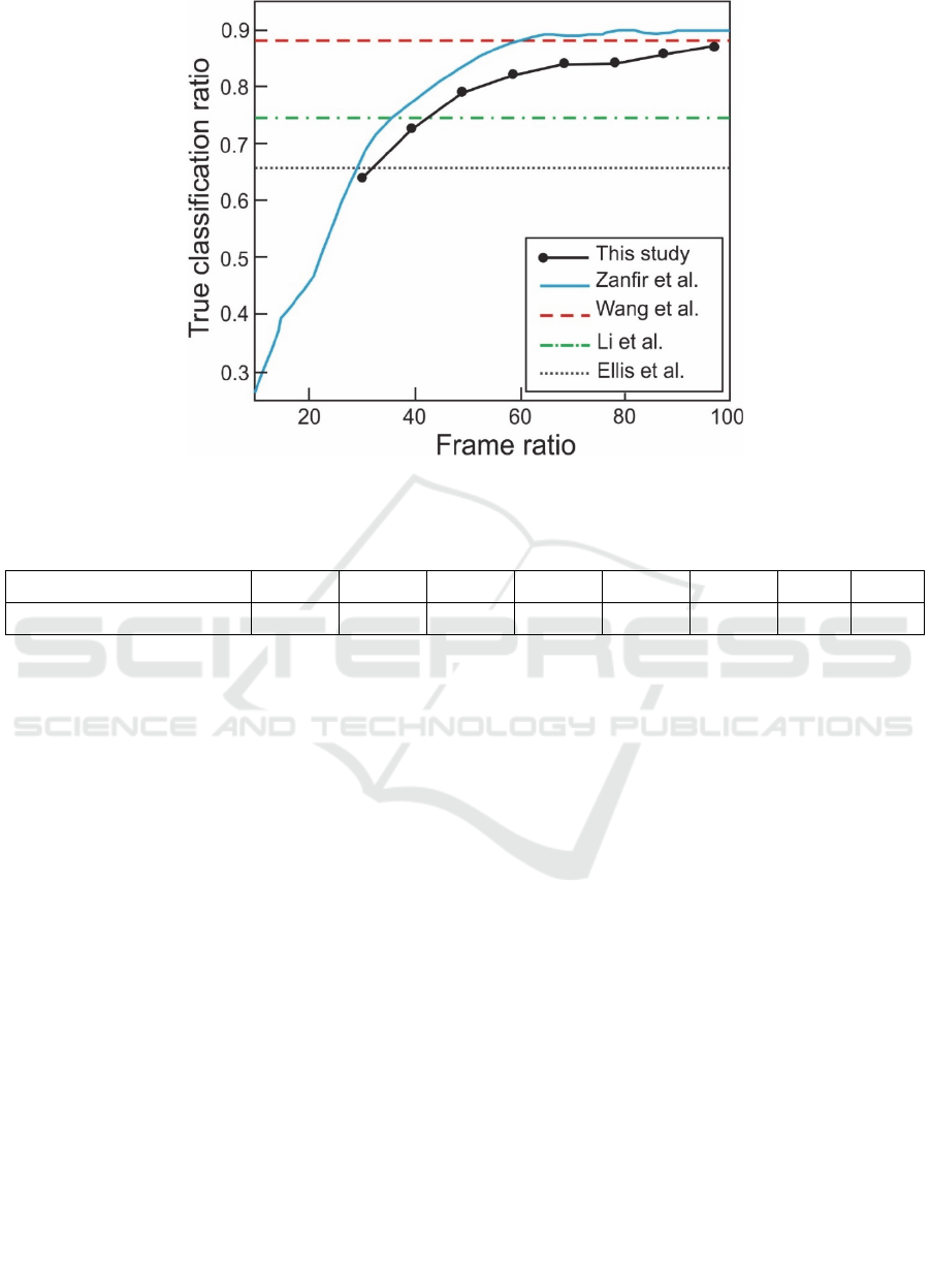
Figure 2: Comparison of the proposed method with the other methods in the literature, (Li et al., 2010; Wang et al., 2012;
Ellis et al., 2013; Zanfir et al., 2013).
Table 1: Cross-Subject test results for different observation ratios.
Observation Ratio
30% 40% 50% 60% 70% 80% 90% 100%
Classification Accuracy
66,34 74,17 80,15 83,11 84,71 84,93 86,51 87,97
with our results. However, they are given here to
show the state of the art in the literature. Only the
method proposed by (Zanfir et al., 2013) is a low
latency method, which can be comparable with out
results.
In the experiments, minimum 30% of the action
sequence is observed. When less than 30% of the
sequence is observed, errors may happen in feature
extraction step. Besides features extracted from a
very limited number of frames is not very distinctive
and classification errors become high. For example,
for a short action sequence, 30% of the sequence
could include only 7-8 frames and features from
these frames could not be sufficient for a successful
classification. For the features obtained from time
series, this situation becomes more significant.
Therefore, we did not tested cases when less than
30% of the action is observed. As it can be seen in
Zanfir et al.’s study, classification ratio is
dramatically low in cases with less than 30% of the
whole sequence is observed. For different
observation ratios cross-subject test results are
shown in Table-1. The proposed method reaches
66,34% classification accuracy when 30% of an
action is observed. Although our method has a lower
success ratio compared with Zanfir et al.’s method,
our method is still comparable with this study.
Furthermore, when the whole sequence is observed,
classification accuracy reaches to 87,97%, which is
more successful than some of the methods in the
literature.
6 CONCLUSIONS
We proposed a low latency action recognition
approach based on depth data. A skeletal model
constructed from depth data is used to extract
features. Some of the features used as time series
while others used as histograms and numeric values.
Although all features help to increase classification
accuracy in our experiments, the features extracted
from time series were very useful when a small part
of the action was observed. Thus, we plan to extend
our future work on obtaining better features from
time series.
REFERENCES
Alpaydin, E., 2004. Introduction to Machine Learning
(Adaptive Computation and Machine Learning), The
MIT Press.
Low Latency Action Recognition with Depth Information
595

Altman, N., 1992. An introduction to kernel and nearest-
neighbor nonparametric regression. The American
Statistician, 46(3), p.175-185.
Ellis, C. et al., 2013. Exploring the trade-off between
accuracy and observational latency in action
recognition. International Journal of Computer Vision,
101(3), p.420-436.
Fothergill, S. et al., 2012. Instructing people for training
gestural interactive systems. In Proceedings of the
2012 ACM annual conference on Human Factors in
Computing Systems - CHI ’12. ACM Press, pp. 1737-
1746.
Freund, Yoav, Robert Schapire, and N. Abe. 1999. "A
short introduction to boosting."Journal-Japanese
Society For Artificial Intelligence 14.771-780, 1612.
Hoai, M. & De La Torre, F., 2014. Max-margin early
event detectors.International Journal of Computer
Vision, 107(2), p.191-202.
Juhl Jensen, L. & Bateman, A., 2011. The Rise and Fall of
supervised machine learning techniques.
Bioinformatics, 27, p.3331-3332.
Keceli A. S., Can A. B., 2014. Recognition of Basic
Human Actions Using Depth Information,
International Journal of Pattern Recognition and
Artificial Intelligence, Vol. 28, No. 02.
Khushaba, R. N., Al-Jumaily, A. & Al-Ani, A., 2007.
Novel feature extraction method based on fuzzy
entropy and wavelet packet transform for myoelectric
Control. 2007 International Symposium on
Communications and Information Technologies.
Li, X., Wang, L. & Sung, E., 2008. AdaBoost with SVM-
based component classifiers. Engineering Applications
of Artificial Intelligence, 21(5), p.785-795.
Li, W., Zhang, Z. & Liu, Z., 2010. Action recognition
based on a bag of 3D points. In 2010 IEEE Computer
Society Conference on Computer Vision and Pattern
Recognition - Workshops, CVPRW 2010. pp. 9-14.
Liaw, A. & Wiener, M., 2002. Classification and
Regression by randomForest. R news, 2, p.18-22.
Shotton, J. et al., 2013. Real-time human pose recognition
in parts from single depth images. Studies in
Computational Intelligence, 411, p.119-135.
Wang, J. et al., 2012. Mining actionlet ensemble for action
recognition with depth cameras. In Proceedings of the
IEEE Computer Society Conference on Computer
Vision and Pattern Recognition. pp. 1290-1297.
Yang, X. & Tian, Y., 2012. EigenJoints-based action
recognition using Naive-Bayes-Nearest-Neighbor. In
Computer Vision and Pattern Recognition Workshops
(CVPRW), 2012 IEEE Computer Society Conference
on. pp. 14-19.
Zanfir, M., Leordeanu, M. & Sminchisescu, C., 2013. The
Moving Pose: An Efficient 3D Kinematics Descriptor
for Low-Latency Action Recognition and Detection.
In Computer Vision (ICCV), 2013 IEEE International
Conference on. pp. 2752-2759.
VISAPP 2016 - International Conference on Computer Vision Theory and Applications
596
