
Adaptive Neuro-Fuzzy Inference System for Echoes Classification in
Radar Images
Leila Sadouki
1,2
and Boualem Haddad
2
1
Institute of Electrical and Electronic Engineering, University M'Hamed Bougara of Boumerdes (UMBB),
Independence Avenue, 35000 Boumerdes, Algeria
2
Laboratory of Image Processing and Radiation, Faculty of Computer Science and Electronics (USTHB),
PObox 32 El Alia. Bab Ezzouar, Algiers, Algeria
Keywords: ANFIS, Image, Radar, Precipitations, Clutter.
Abstract: In order to remove the undesirable clutter which reduces the radar performances and causes significant
errors in the rainfall estimation, we implemented in this paper an algorithm deals with the classification of
radar echoes. The radar images studied are those recorded in Sétif (Algeria) every 15 minutes, we used a
combination of textural approach, with the grey-level co-occurrence matrices, and a grid partition based
fuzzy inference system, named ANFIS-GRID. We have used two parameters, namely Energy and local
homogeneity that are considered to be the most effective in discriminating between precipitation echoes and
clutter. Those parameters are used as inputs for the ANFIS-GRID, while the output of this system is the
radar echo types. In function of the best mean rate of correct recognition and using two different
optimization methods, the structure with 2 inputs, 4 membership functions, 16 rules and 1 output was
selected as the most efficient ANFIS-GRID. This method gives a mean rate of correct recognition of echoes
to over 93.52% (91.30% for precipitation echoes and 95.60% for clutter). In addition, the proposed
approach gives a process maximum time of less than 90 seconds, which allows the filtering of the images in
real time.
1 INTRODUCTION
The demands for finer scale meteorological services
have more and more required higher resolution
observations to initialize and evaluate weather and
climate models, applications, and products. In
response to these demands smart techniques are
increasingly used in the design, classification,
modeling and control of complex systems, such as
neural networks, fuzzy logic and genetic
algorithms…
For weather radar, the presence of echoes
coming from the earth's surface, or clutter, mixed
with precipitation echoes, making the hydrological
measurement very difficult (Sauvageot and
Despaux, 1990), a good way to eliminate clutter is to
compare the statistical properties of the ground
echoes to those of precipitations echoes, such as
textural features (Haddad et al., 2004). The most
common techniques used are Doppler filtering
(Doviak and Zrnic, 1993), or dual polarization
filtering (Islam et al., 2012; Chandrasekar et al.,
2013). Clutter can be removed by analyzing in real
time the coefficient of the autocorrelation function
of the radar signal (Hamuzu and Wakabayashi,
1991). Others applied the fuzzy logic technique, to
classify the Doppler radar echoes types (Hubbert et
al., 2009) or for identifying non-precipitating echoes
in radar scans (Berenguer et al., 2006; Cho et al.,
2006). In (Sadouki and Haddad, 2013), they
combined the textural properties of the echoes with
the fuzzy approach in order de classify the echoes.
Furthermore, (Xiang, 2010) used the neuro-fuzzy
approach to eliminate noise in Doppler radar signals.
Depending on the on above literature survey, it’s
interesting to implement an algorithm which
combines the textural features, based on the method
of grey-level co-occurrence matrices, and an
Adaptive Neuro-Fuzzy System (ANFIS) with grid
partition. The input variables for our system are two
textural parameters considered as effective elements
for distinguishing between precipitation echoes and
clutter (Sadouki and Haddad, 2013). This method
was applied to the images taken in the region of
Sétif (Algeria).
Sadouki, L. and Haddad, B.
Adaptive Neuro-Fuzzy Inference System for Echoes Classification in Radar Images.
DOI: 10.5220/0005717401590166
In Proceedings of the 11th Joint Conference on Computer Vision, Imaging and Computer Graphics Theory and Applications (VISIGRAPP 2016) - Volume 4: VISAPP, pages 159-166
ISBN: 978-989-758-175-5
Copyright
c
2016 by SCITEPRESS – Science and Technology Publications, Lda. All rights reserved
159
The remainder of the paper is organized as
follows: Section 2 focuses on database used in this
work, sections 3 and 4 deal respectively with the
used concepts and the data processing. We illustrate
discuss and validate the different results in sections
5 and 6. Finally, and in section 7, we give our
conclusion.
2 DATA BASE
Weather radar of Sétif is of the Type AWSR-81
(Algerian Weather Service Radar). It is non-coherent
pulsed radar which consists of a transmitter, a
receiver, a duplexer, antenna of 3 m in diameter and
is associated with a SANAGA chain (Système
d’Acquisition Numérique pour l’Analyse des Grains
Africains) which is a system of acquisition and
digitization of images (Sauvageot and Despaux,
1990). The main characteristics of this radar are:
Transmission power: 250 kW;
Transmission frequency: 5.6 GHz;
Reception sensitivity to: -110 dBm;
Pulse width: 2μs;
Antenna gain: 30 dB;
Return period: 4 ms;
Beam width (3 dB): 1.1;
Our database consists of images taken during the
period of 1997-2001. Sétif radar is positioned at
latitude of 36°11'N, a longitude of 5°25' E and an
altitude of 1700 m above the sea level. It records
every fifteen minutes an image of 512×512 pixels
using the PPI (Plan Position Indicator) presentation,
with a resolution of 1 km per pixel.
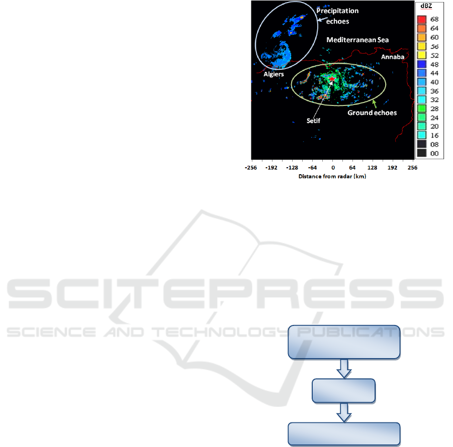
As shown in the image of Figure 1, the images
recorded in this site using the C-band meteorological
radar, use a palette of sixteen colors. We find in
those images a lot of ground echoes coming from the
earth's surface. These echoes are, in particular, due
to the fact that Sétif region is a part of the Algerian
highlands and its Radar is surrounded by several
ground obstacles. The nearest ground echoes are
produced largely by the industrial area. Beyond the
horizon, the ground obstacles produce several
ground echoes in the radar images. For example, to
the southwest, 60 km away from the radar, there are
the mountains of Djurdjura, which reach an altitude
of 2300 m. In the same direction, 40 km away from
the radar, we find the mountains of Bibans with a
height of 1417 m. To the northeast, at a shorter
distance (about 30 km away from the radar), are
located the mountains of Babors, which reach an
altitude of 2004 m.
Figure 1: Radar images of Sétif.
3 USED CONCEPTS
The main methods that are considered in this paper
are textural approach, using the co-occurrence
matrices, and the Neuro-Fuzzy controller. The latter,
is the combination of the Neural networks and Fuzzy
logic, that takes advantages of both approaches.
Figure 2 summarizes the concepts used in this study.
Figure 2: Block diagram of the used concepts.
3.1 Co-occurrence Matrices
The grey-level co-occurrence matrices are among
the most frequently used statistical methods in the
field of the texture analysis of the radar and the
satellite images (Haralick, 1979). The gray-level Co-
occurrence matrix of an image is obtained by
estimating the joint conditional density of
probability functions of second-order P (i, j / d, θ ),
the latter represents the transition probability of a
pixel of gray level “i” to a pixel of gray level “j”.
Input: Features extraction
from the Radar images
ANFIS
Output: Class identification
VISAPP 2016 - International Conference on Computer Vision Theory and Applications
160

This transition is controlled by: the distance “d”
between the two pixels and the orientation “θ”which
is defined by the angle between the direction of
transition and the image scanning direction.
The orientation “θ” can be determined also with
Cartesian coordinates (Δx, displacement in the
horizontal direction and Δy, displacement in the
vertical direction)
The elements P (i, j) denoted Pij of the Co-
occurrence matrix represent the frequency of
occurrence of the pair of gray levels (i, j) in the
processing window “W” of T1×T2 size, according to
a relationship represented by the pair (Δx, Δy). They
are defined as follows:
P (i , j /Δx ,Δy) = Card { (m ,n), ( m+Δx ,
n+Δy)∈ W/ I( m , n) = i and I ( m +Δx , n
+Δy) = j }
(1)
Where Card, is the cardinal or the number of
elements, and I (m, n) and I (m+Δx, n+Δy) represent
respectively the intensities of pixels “i” and “j”
located at (m,n) and (m+Δx, n+Δy) in the window
“W”.
The elements of the direction matrix C
ij
(θ, d) are
written:
C
i
j
(θ,d) = P (i , j /
Δ
x , Δy) / r
(2)
Where “r” is the normalization parameter which is
equal to: (T1-|Δx|) × (T2-|Δy|).
There are eight Co-occurrence matrices C (θ, d)
for different directions (θ = 0°, 45°, 90°, 135°, 180°,
225°, 270°, 315°).
We can calculate, using the Co-occurrence
matrix, a set of statistical properties (i.e. Mean,
Variance, Inertia, Local homogeneity, Energy,
Correlation, Entropy, Nuances grouping, and
Predominance grouping), which allow us to reveal
the particular characteristics of image texture. In this
paper, we will use only two parameters (i.e. Local
homogeneity and Energy) that give the results the
most uncorrelated, with the direction θ =0° and the
distance d=1, which correspond to the Cartesian
coordinates (Δx=0, Δy=1) (Sadouki and Haddad,
2013).
It’s worth noting that, among the values of d=
{1,2,3,4}, the distance d = 1, was chosen, by
experience, as the best value in terms of
effectiveness (in distinguishing between
precipitation echoes and clutter) and the
proportionality with the size of the study windows
(5×5 pixels window).
Equations of those parameters are: (Haralick,
1979; Unser, 1986; Peckinpaugh, 1991).
Energy which measures textural uniformity:
−
=
−
=
=
1
0
1
0
2
gg
N
i
N
j
ij
CE
(3)
The local homogeneity that gives greater weight
to the occurrence frequencies of homogeneous
zones:
()
()
[]
−
=
−
=
−+=
1
0
1
0
2
1
gg
N
i
N
j
ijL
CH ji
(4)
3.2 Neuro-Fuzzy Concept
A Neuro-Fuzzy (NF) system is a combination of
Artificial Neural Network (ANN) and Fuzzy
Inference System (FIS) in such a way that ANN
learning algorithms are used to determine the
parameters of FIS (Kurian et al., 2006).
ANFIS (Adaptive Neuro-Fuzzy Interface
System) is the fuzzy Sugeno model based paradigm
that grasps the learning abilities of ANN to enhance
the intelligent system’s performance using a priori
Knowledge.
Using a given input/output data set, ANFIS
constructs a fuzzy inference system (FIS) whose
membership function parameters are tuned using
either a back-propagation algorithm alone, or in
combination with a least squares method. This
allows your fuzzy systems to learn from the data
they are modeling. The learning method works
similarly to that of neural networks (Chaudhari et
al., 2012). In fact, ANFIS cancels out the
interference and gives better performance even if the
complexity of the signal is very high.
We used in this paper, the ANFIS-GRID fuzzy
inference system which is the combination of grid
partition and ANFIS. Grid partition divides the data
space into rectangular sub-spaces using axis-
paralleled partition based on predefined number of
membership functions and their types in each
dimension as shown in Figure 3.
Figure 3: Grid partition of an input domain with 2 input
variables and 2 membership functions for each input.
Adaptive Neuro-Fuzzy Inference System for Echoes Classification in Radar Images
161

The number of fuzzy rules increases
exponentially when the number of input variables
increases. For example, if there are averagely “m”
membership functions (MF) for every input variable
and a total of “n” input variables for the problem, the
total number of fuzzy rules is “m
n
” (Wei et al.,
2007).
For a first-order Sugeno fuzzy model, a common
rule set with “k” fuzzy “if-then” rules is given by:
(Bhavani et al., 2012)
Rule k:
If X is Ai and Y is Bj,
Then fk = pk X + qk Y + rk
Where: k=1...i*j
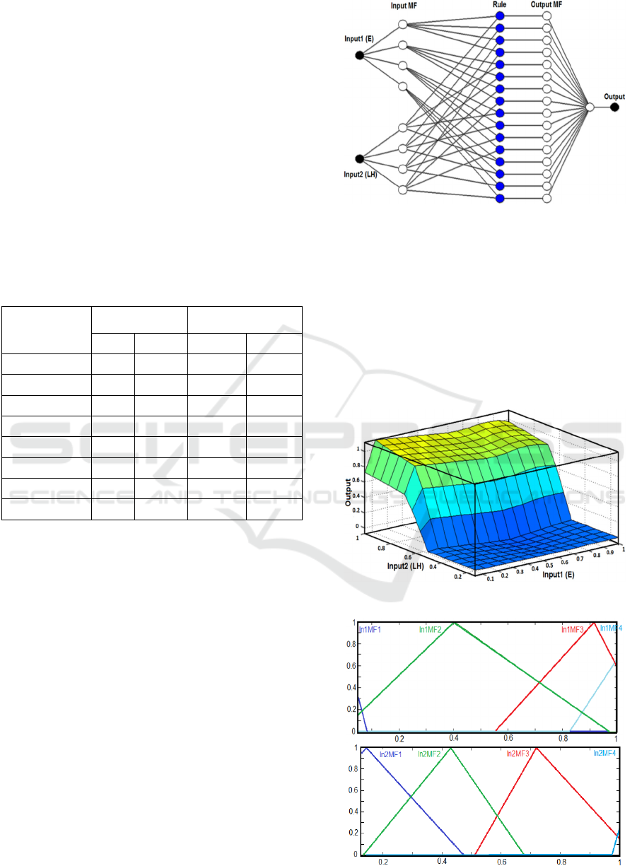
To present the ANFIS architecture, let us
consider the example of the Figure 4 which has two
inputs (X , Y), and one output “f”.
Layer 1: Calculate Membership Value for Premise
Parameter: Every node “i” in this layer is an
adaptive node
Layer 2: Firing strength of rule: The nodes in this
layer are fixed (not adaptive).These are labeled “
Π”
to indicate that they play the role of a simple
multiplier.
Layer 3: Normalize firing strength: Nodes in this
layer are also fixed nodes. These are labeled “N” to
indicate that these perform a normalization of the
firing strength from previous layer.
Layer 4: Consequent Parameters: All the nodes in
this layer are adaptive nodes.
Layer 5: Overall output: This layer has only one
node labeled “Σ” indicated that is performs the
function of a simple summer.
Figure 4: ANFIS Architecture (an example with 2 inputs
and 4 rules).
4 DATA PROCESSING
To classify the types of echoes in radar images, a
variety of samples (sub-image), carefully selected
from images, where precipitation echoes (class 1)
are distinctly separated from the ground echoes
(class 2). It’s important to note that each sub-image,
of a maximum size of about 15×15 pixels, illustrates
a different meteorological situation.
For each 5×5 pixels window in a given sub-
image, we calculated the statistical parameters
Energy and Local homogeneity that have been found
to be useful in discriminating between precipitations
and clutter, and have been chosen as inputs of our
classifier. (Sadouki and Haddad, 2013)
As result to the previous process, we were
capable to construct our database of 1000 vectors
that corresponds to our two classes, 500 for clutter
and 500 for precipitations. Each vector is composed
of 3 elements, Energy, Local homogeneity and class.
In fact, we used MATLAB commands for
learning process with 1000 epochs and 600 training
sample from the two classes. In addition, the
optimization methods applied, in order to train the
membership function’s parameters to emulate the
training data, are the back-propagation and the
hybrid methods, where the second method is a
combination of least-squares and back-propagation
gradient descent method.
It’s worth mentioning that the others 400 vectors
of our data base were use in the testing process.
The output of the ANFIS classifier will be used
later to find an appropriate approach, which will
allow us to separate the ground echoes from the
precipitation echoes in order to eliminate the
undesirable echoes.
5 RESULTS AND DISCUSSION
After creating different architectures of ANFIS
classifier, and using triangular membership
functions for each Input, we perform the training of
each classifier using our database. Since the errors,
obtained during training and testing, seem to be of
the same level, so, we were obliged to validate our
classifier. Thus, we classified 20 images using 8
different topologies, after that, we calculated the rate
of correct recognition for each image (denoted
RCR). This rate is calculated by the following
expression:
100)N
X
(RCR
c
1i
i
×=
=
(5)
VISAPP 2016 - International Conference on Computer Vision Theory and Applications
162
Where:
c : Is the number of classes.
N : Is the total number of pixels.
Xi : Is the number of pixels correctly classified to
the class i.
Table 1 collects the results obtained, with
different topologies and by changing:
The number of Membership Functions for each
input (MFin1-MFin2),
Rules.
Optimization Method.
Where, MFin1 and MFin2 are the number of
membership functions for the parameters Energy
and local homogeneity respectively.
Table 1: Rate of correct recognition (RCR in %) and the
associated time (in Seconds) for different topologies and
different optimization methods (average of 20 images).
Topology
(MFin1-MFin2)
Back propagation
Opt. Method
Hybrid Opt. Method
RCR Time RCR Time
(2-2) 92,85 71.30 92,65 72.14
(3-3) 92,96 71.61 92,22 73.13
(4-4) 93,52 72.14 92,57 74.93
(5-5) 90,60 73.25 91,95 75.78
(6-6) 83,89 73.78 92,30 76.70
(7-7) 79,42 74.84 92,88 77.19
(10-10) 75,37 76.28 88,52 80.40
(15-15) 73,11 78.67 87,16 81.23
According to the results of the Table 1, it’s clear
that from the topology (5-5) and when we use the
back propagation method, the RCR decreases with
the increasing of the number of the membership
functions, but for the hybrid method, the same rate
decreases from the level (7-7). Also, we can see that
the most adequate topology, which was fixed after
several trials based on the best rate of correct
recognition, is the (4-4) network with the back
propagation optimization method, with 2 inputs, 4
membership functions, 16 rules and 1 output. In
addition the processing time is less than 90 seconds,
which is a relatively small time comparing with the
image acquisition time.
The model of this ANFIS is shown in Figure 5.
Rules:
Rules 1 to 4: with i,j=1..4
If (Input1 is In1MF1) and (Input2 is In2MFi)
then (Output is OutMFj)
Rules 5 to 8: with i=1..4 and j=5..8
If (Input1 is In1MF2) and (Input2 is In2MFi)
Figure 5: ANFIS Structure.
then (Output is OutMFj)
Rules 9 to 12: with i=1..4 and j=9..12
If (Input1 is In1MF3) and (Input2 is In2MFi)
then (Output is OutMFj)
Rules 13 to 16: with i=1..4 and j=13..16
If (Input1 is In1MF4) and (Input2 is In2MFi)
then (Output is OutMFj)
Where, OutMFj (j=1..16) are the membership
functions of the outputs.
Figure 6: ANFIS Surface View.
Figure 7: Membership functions plot (final forms).
Adaptive Neuro-Fuzzy Inference System for Echoes Classification in Radar Images
163
The ANFIS surface view and the final forms of
the 4 membership functions of each input are shown
in Figure 6 and Figure 7 respectively. Where,
In1MFi (i=1..4) are the membership functions of the
first input Energy or “E”, while In2MFi are the
membership functions of the second input Local
Homogeneity or “HL”.
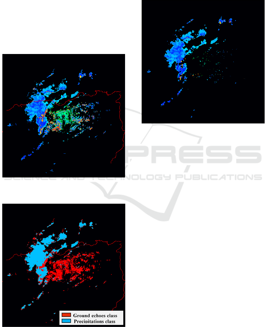
As illustration of the output of our classifier, the
image of Figure 8 recorded in 09 November 2001 is
considered. It provides the case were the
precipitations partially cover the ground echoes.
Figure 8: Radar image of Sétif region recorded in
09/11/2001.
Figure 9: Radar image of Sétif region (Classified image).
In order to eliminate the undesirable echoes or
clutter, we used our approach, to classify and filter
this image with the (4-4) ANFIS network. To do
that, we performed the following process:
Figure 10: Radar image of Sétif region (Filtered image).
For each pixel in the image and using the surrounded
pixels, we computed the parameters Energy and
Local homogeneity, after that, we applied them to
the ANFIS network to get, as result, the appropriate
class for that pixel. With this classifier, we can
observe clearly through Figure 9 that the two classes
are well classified.
Whereas for the filtering, and for each pixel in
the image, we performed the following test: If the
current pixel is evaluated in the class of clutter, we
assign the black colour for that pixel, otherwise, we
maintain the initial colour. Figure 10 shows that the
ground echoes appearing on the considered image of
Sétif are eliminated and the precipitation fields are a
little bit affected by the filtering.
6 VALIDATION
It’s very important to note that for the case of
images, where the precipitations cover partially the
ground echoes, the estimations of the
RCR
in the
images, are very difficult. Consequently, we were
obliged to use another way to validate our technique,
which is the estimation of the intensity of rainfall
using the radar relationship for temperate climates:
(Sauvageot, 1992)
Z = 300 R
1.5
(6)
VISAPP 2016 - International Conference on Computer Vision Theory and Applications
164

Where Z and R are, respectively, the radar
reflectivity factor (expressed in mm
6
m
−3
) and the
precipitation rate (expressed in mm h
−1
).
To verify that the filtering of clutter does not
affect the reflectivity of precipitation echoes, we
compared the intensity of rainfall collected and
measured by pluviometer, and that estimated by
radar images during the extreme rain event,
observed on November 09-10, 2001 in the region of
Algiers, which was at the origin of a natural disaster.
We recorded in the day of November 10
th
an
amount of rain equals to 132 mm in 6 hours duration
(6:00 to 12:00). (Haddad et al., 2003)
Since we have a chronological set of 25 images
recorded from 6:00 am to 12:00 pm, we were
capable to find the intensity of rainfall estimated by
the filtered radar images which is 121.6 mm. Thus,
the estimation error is about 7.87%.
7 CONCLUSIONS
The method described in this paper shows that the
combination of the textural features, using Co-
occurrence matrices, and Adaptive Neuro-Fuzzy
Interface System, with the utilization of grid
partition, allows an efficient radar echoes
classification. In function of two factors which are
filtering rate and computation time, the structure 2
inputs with 4 membership functions for each and 16
(or 4
2
) rules was selected as the most efficient
network. The application of this approach gives a
mean rate of correct recognition of echoes to over
93.52% (91.30% for precipitation echoes and
95.60% for clutter) for the images recorded in the
site of Sétif. In addition, time of processing is about
90s which is less than 2 minutes. It would be
interesting to extend this study to other sites of
different climates to check the effectiveness of the
technique and if the thresholds and membership
functions always stay invariant.
ACKNOWLEDGEMENTS
The authors would like to thank the National
Meteorology Office of Algeria for providing the
radar data base used in this study. We would also
like to thank the reviewers for their valuable
comments and suggestions.
REFERENCES
Berenguer, M., Sempere-Torres, D., Corral, C. and
Sanchez-Diezma, R., 2006. A fuzzy logic technique
for identifying nonprecipitating echoes in radar scans.
Journal of Atmospheric and Oceanic Technology, vol.
23, pp. 1157-1180.
Bhavani Sankar, A., Kumar, D., and Seethalakshmi, K.,
2012. A New Self-Adaptive Neuro Fuzzy Inference
System for the Removal of Non-Linear Artifacts from
the Respiratory Signal. Journal of Computer Science.
vol. 8 (5), 621-631.
Chandrasekar, V., Keränen, R., Lim, S., and Moisseev, D.,
2013. Recent advances in classification of
observations from dual polarization weather radars.
Atmospheric Research, vol. 119, pp. 97-111.
Chaudhari, O. K., Khot, P. G., Deshmukh, K. C., and
Bawne, N. G., 2012. ANFIS based model in decision
making to optimize the profit in farm cultivation.
International Journal of Engineering Science and
Technology (IJEST). Vol. 4 (2), 442-448.
Cho, Y. H., Lee, G., Kim, K. E. and Zawadzki, I., 2006.
Identification and removal of ground echoes and
anomalous propagation using the characteristics of
radar echoes. Journal of Atmospheric and Oceanic
Technology. vol. 23, pp. 1206-1222.
Doviak, R. J., and Zrnic, D. S., 1993. Doppler radar and
weather observations, Academic Press., pp. 562.
Haddad, B., Sadouki, L., Naili, R, Adane, A., and
Sauvageot, H., 2003. Analyse De La Dimension
Fractale Des Echos De Precipitations: Cas Des
Inondations D'Alger. Publication de l 'Association
Internationale de Climatologie. vol. 15, pp.386-392.
Haddad, B., Adane, A., Sauvageot, H., and Sadouki, L.,
2004. Identification and filtering of rainfall and ground
radar echoes using textural features. International
Journal of Remote Sensing. vol. 25(21), pp. 4641–
4656.
Hamuzu, K., and Wakabayashi, M., 1991. Ground clutter
rejection. In Hydological applications of Weather
Radar, Clukie and Collier. Ed Ellis Horwood Ltd, pp.
131–142.
Haralick, R. M., 1979. Statistical and structural
approaches to textures. Proceedings of the IEEE on
Image Processes, vol. 67, pp. 786–804.
Hubbert, J. C., Dixon, M., and Ellis, S. M., 2009. Weather
Radar Clutter. Part II: Real-Time identification and
filtering. Journal of Atmospheric and Oceanic
Technology, vol. 26, pp. 1181–1197.
Islam, T., Rico-Ramirez, M. A., Han, D. and Srivastava,
PK., 2012. Artificial Intelligence Techniques for
Clutter Identification with Polarimetric Radar
Signatures. Atmospheric Research, 109-110, pp. 95-
113.
Kurian, C. P., George, V. I., Jayadev, B., and
Radhakrishna, S. A., 2006. ANFIS Model For The
Time Series Prediction of Interior Daylight
illuminance. AIML Journal. Vol. 6 (3).
Peckinpaugh, S. H., 1991. An Improved Method for
Computing Grey-Level Co-Occurrence Matrix Based
Adaptive Neuro-Fuzzy Inference System for Echoes Classification in Radar Images
165

Texture Measures. CVGIP: Graphical Models and
Image Processing. vol. 53, 574–580.
Sadouki, L., and Haddad, B., 2013. Classification of radar
echoes with a textural–fuzzy approach: an application
for the removal of ground clutter observed in Sétif
(Algeria) and Bordeaux (France) sites. Int. J. of
Remote Sensing, vol. 34(21), 7447-7463.
Sauvageot, H., and Despaux, G., 1990. SANAGA: Un
système d’acquisition numérique et de visualisation
des données radar pour la validité des estimations
satellitaires de précipitations. Veille Climatique
Satellitaire, vol. 31, pp. 51–55.
Sauvageot, H., 1992. Radar Meteorology. Norwood:
Artech House., pp. 361.
Unser, M., 1986. Sum and difference histograms for
texture classification. IEEE Transactions on Pattern
Analysis and Machine Intelligence. vol. 8(1), pp. 118–
125.
Wei, M., Bai, B., Sung, A. H., Liu, Q., Wang, J., and
Cather, M. E., 2007. Predicting injection profiles using
ANFIS. Information Sciences. vol. 177, 4445–4461.
Xiang, L., 2010. Adaptive Network Fuzzy Inference
System Used in Interference Cancellation of Radar
Seeker. IEEE International Conference on Intelligent
Computing and Intelligent Systems (ICIS). vol. 2, pp.
93–97.
VISAPP 2016 - International Conference on Computer Vision Theory and Applications
166
