
Re-parameterization of a Deformation Model for Non-rigid Registration
Van-Toan Cao, Trung-Thien Tran and Denis Laurendeau
Computer Vision and Systems Laboratory, Department of Electrical and Computer Engineering,
Faculty of Science and Engineering, Laval University, 1065 Avenue of Medicine, Quebec (QC), G1V 0A6, Canada
Keywords:
Non-rigid Registration, Deformation, Correspondence, Alignment, Parameterization.
Abstract:
In this paper we present a method for non-rigid registration of meshes. The method aligns two surfaces of
deformable objects by automatically separating the deformation into a single global transformation and other
local deformations. The local deformations are found by applying the deformation model proposed by Sumner
(Sumner et al., 2007) that previous methods have used to register two surfaces. However, we specify a rigid
transformation for each node of the deformation graph using a rotation matrix and a translation vector. With
this model, unit quaternions of rotation matrices are paramterized using an homeomorphic relation between
the 4D unit sphere and the 3D projective space. Therefore, the number of unknowns is reduced by half
compared to the original models based on affine transformations and the optimization process is less complex.
We demonstrate the efficiency of the proposed method by aligning the surfaces of data sets without any prior
knowledge and assumptions about the deformation between the two surfaces.
1 INTRODUCTION
With the availability of depth cameras (e.g. Microsoft
Kinect and similar RGB-D sensors), obtaining 3D
data is simpler and more flexible. Moreover, these
cameras capture 3D data at a high frame rate (i.e.
about 30 frames/second) and allow the scanned dy-
namic objects (e.g. human body, animals) to be un-
constrained during the scanning process. In contrast,
the acquired data is also more complex to process
due to noise and outliers as well as object deforma-
tion between scans. Non-rigid registration applied on
deformable objects is the task of finding a mapping
between two scans and transforming the source scan
into the target scan. This process is an essential step
in the applications such as 3D tracking, 3D model re-
trieval, 3D reconstruction and 3D animation.
Because the object can deform its shape between
different scans, rigid registration cannot be applied
to align two scans together. Rigid registration meth-
ods find only a single global rigid transformation and
cannot solve for other local deformations. There-
fore, non-rigid registration is required for dynamic
objects since it solves for both global transformation
and other local deformations. However, this task is
still a difficult and ill-posed problem due to high-
dimensional search space of parameters. Various
methods impose constraints to transform the problem
into a well-posed one. For example, a template can be
used as prior geometry, it can be assumed that the mo-
tion between two scans is small, artificial markers can
be used as initial correspondences or the deformation
can be approximately isometric.
In this paper, we present a method to align two
surfaces of scanned dynamic objects without any
prior knowledge on the deformation between scans
or without simplifying assumptions either. Inspired
by the method of (Cao et al., 2015) (sometimes re-
ferred to as TSA in this paper), which efficiently
solves the non-rigid registration under large defor-
mation between the surfaces, the method first finds a
single global transformation and then optimizes other
local deformations based on the deformation model
proposed by Sumner (Sumner et al., 2007). How-
ever, the previous work is only applied on the sur-
faces for which a single patch of continuously con-
nected triangular mesh is presented in order to com-
pute geodesic distances when generating a graph of
deformation model. The method proposed here also
performs well on surfaces composed of different dis-
connected patches (as shown in Fig. 4) because the
graph is created using the Euclidean distance. More-
over, the previous work uses twelve parameters for
each node’s affine transformation in the deformation
graph. This causes the cost function to be complex
and the solution space to be very large. The current
work only specifies six parameters for each node in
which three parameters are used for each translation
Cao, V-T., Tran, T-T. and Laurendeau, D.
Re-parameterization of a Deformation Model for Non-rigid Registration.
DOI: 10.5220/0005714300370047
In Proceedings of the 11th Joint Conference on Computer Vision, Imaging and Computer Graphics Theory and Applications (VISIGRAPP 2016) - Volume 1: GRAPP, pages 39-49
ISBN: 978-989-758-175-5
Copyright
c
2016 by SCITEPRESS – Science and Technology Publications, Lda. All rights reserved
39

vector and each unit quaternion associated with each
rotation matrix is parameterized completely by three
parameters. With this improvement, the number of
unknowns is reduced by half while the as-rigid-as-
possible regularization for each node is achieved au-
tomatically. Consequently, the problem of non-rigid
registration is better formulated in order to find the
optimal solution.
2 RELATED WORK
Non-rigid registration is an emerging field in com-
puter vision and computer graphics. In this section,
we only review the state-of-the-art works that are the
most relevant to our method.
In the process of 3D scanning of objects, holes,
outliers and noise are inevitable issues of the acquisi-
tion process. So, to create a complete model, a tem-
plate which has the same topology as the object is
used as a prior geometry before being merged into the
scanned data. The template can be a generic model
(Allen et al., 2003; Zhang et al., 2004; Amberg et al.,
2007) or it can be obtained during a static acquisition
phase (Li et al., 2009; Zollh
¨
ofer et al., 2014). Be-
cause the templates may not be available for all types
of models, the methods in (Chang and Zwicker, 2008;
Huang et al., 2008; Sagawa et al., 2009; Cao et al.,
2014) assume that local deformations are small to val-
idate local feature descriptors used for finding some
initial correspondences between the two surfaces in
order to guide the registration process.
Applying the deformation model proposed by
Sumner (Sumner et al., 2007), the methods in (Li
et al., 2008; Li et al., 2013; Zeng et al., 2013; Zhang
et al., 2014; Dou et al., 2015) register the deformation
graph of the source surface with the target surface.
Each node’s displacement is specified by the twelve
parameters of an affine transformation. Once the de-
formation graph aligns with the target surface, the re-
maining data of the source surface is transformed us-
ing linear blending-based interpolation. These meth-
ods require that the motion between the two surfaces
to be aligned is small to avoid tangential drift during
the optimization process. When the motion between
two surfaces is large, a rigid transformation between
them is required for the above techniques to work.
Instead of using affine transformations for points
(nodes) of a sparsely sampled set, the methods in
(Bonarrigo et al., 2014; Newcombe et al., 2015) spec-
ify only rigid transformations for these points and
then use dual-quaternion blending for the interpola-
tion step. The optimization process in (Newcombe
et al., 2015) searches for the parameters of a global
rigid transformation and other local rigid transforma-
tions at each iteration. This strategy can cause the
optimization to converge to a wrong minimum if the
motion between the two surfaces is large. The work of
(Bonarrigo et al., 2014) assumes that some initial cor-
respondences are available before running the opti-
mization. In approaches based on the signed distance
field, the methods in (Rouhani et al., 2014; Zhang
et al., 2015) do not need to find any correspondences
for the registration process. However, these methods
provide misalignment results when the surfaces are
not watertight and clean due to the presence of holes,
outliers or noise.
Some methods are based on probabilistic ap-
proaches for non-rigid registration. In (Myronenko
and Song, 2010), Gaussian Mixture Model centroids
(source set) are fitted to the data (target set) by maxi-
mizing the likelihood function. The registration prob-
lem is thus considered as a probability density esti-
mation. In another work, the algorithm in (Jian and
Vemuri, 2011) minimizes the statistical discrepancy
measure between two Gaussian mixture models in
which each model represents a point set. These meth-
ods impose a large-complex computational burden to
identify the correspondences and local deformations.
They are almost only applied to 2D data or small 3D
data sets. In (Anguelov et al., 2004), a Markov Ran-
dom Field optimization is formulated to establish the
correspondences and find rigid local transformations
between the two surfaces. Assuming that the geodesic
distance between any two points is preserved before
and after deformation and that the source surface is a
subset of the target surface, the method can align the
surfaces under large deformation.
3 REGISTRATION METHOD
3.1 Parameterization of Rotation
3D rotations are applied in algorithms in the context
of computer vision and computer graphics to describe
the transformations of objects under both rigid and
non-rigid motion. Although a 3D rotation matrix has
nine elements, it only has three degrees of freedom
(DOF). When an algorithm uses an optimization pro-
cess to find the parameters of such a matrix, it is im-
portant to use a minimal parameterization that reduces
the computational burden and makes the calculation
of derivatives relating to rotation matrix simpler.
Compared to other common parameterizations
such as Euler angles and axis-angle representation,
unit quaternion is preferable because it avoids am-
biguous configurations such as gimbal lock. Although
GRAPP 2016 - International Conference on Computer Graphics Theory and Applications
40
a unit quaternion has four elements, it has only three
DOF due to the unit norm constraint. In the optimiza-
tion process, an efficient parameterization of a unit
quaternion should use only three parameters, these
three parameters should be allowed to change arbi-
trarily by the optimization process and the unit norm
constraint should be satisfied automatically (Schmidt
and Niemann, 2001).
From the above discussion, a unit quaternion pa-
rameterization of the rotation matrix proposed in
(Terzakis et al., 2012) by exploiting the homeomor-
phic relation between the 4D unit sphere and the 3D
projective space is exploited in our optimization pro-
cess (section 3.2.2). The unit quaternion parameteri-
zation is described as follows.
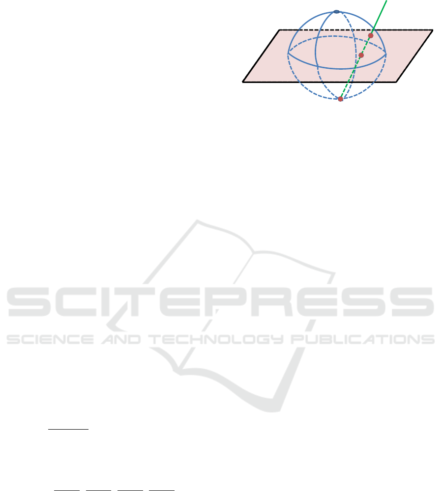
As shown in Fig. 1, we assume that there is a unit
quaternion q = (q
0
,q
1
,q
2
,q
3
) where q
0
is the real part
and (q
1
,q
2
,q
3
) are the imaginary parts. This quater-
nion can be considered as a hypersphere in 4D space
and described by:
q
2
0
+ q
2
1
+ q
2
2
+ q
2
3
= 1 (1)
Let S = (0,0,0,−1) be the south pole in this 4D
sphere and π be the 3D equatorial hyperplane contain-
ing the origin of R
4
. Let now r(t), parameterized by t,
be the ray from S that passes through any point (x, y,z)
of the equatorial plane:
r(t) = (0,0,0,−1) +t[x y z 1]
T
(2)
The ray intersects the surface of the sphere at P.
So, P is back-projected on π through the ray. Because
P lies on both the sphere and the ray, its coordinates
satisfy the following equation:
(tx)
2
+ (ty)
2
+ (tz)
2
+ (t − 1)
2
= 1 (3)
From Eq. 3, t is obtained in terms of parameters
x,y, z: t =
2
1+x
2
+y
2
+z
2
. Finally, by substituting the
value of t into Eq. 2, one obtains the coordinates of
a unit quaternion in x,y, z.
q =
2x
1 + α
2
,
2y
1 + α
2
,
2z
1 + α
2
,
1 − α
2
1 + α
2
(4)
where α
2
= x
2
+ y
2
+ z
2
With this parameterization, a rotation matrix R is
obtained by using only three parameters (x,y, z) when
combining Eq. 4 and Eq. 17 (as described in the Ap-
pendix). Therefore, in an optimization process, we
do not need to impose a unit-norm constraint for a
quaternion. This paramterization is specially desired
when the number of optimized parameters is large as
in non-rigid registration.
S
P
(x,y,z)
r(t)
π
Figure 1: The 4D spherical hypersurface of unit quaternions
pictured as a 3D sphere. Point S is the center of projection,
(x,y,z) a point on the 3D equatorial hyperplane. The ray
r(t) intersects the surface of the sphere at P (Terzakis et al.,
2012).
3.2 Non-rigid Registration
3.2.1 Deformation Model
The presented work is derived from the methods in
(Sumner et al., 2007) and (Cao et al., 2015). For com-
pleteness, in this section, the main idea of the previ-
ous work is described and the changes are presented
in the new algorithm (for more details, we refer the
reader to the work in (Sumner et al., 2007; Cao et al.,
2015)).
To register the source surface with the target sur-
face, a graph of the deformation model is generated
by sampling the source surface. Then, a 3D point of
the graph is called a ‘node’ g
j
( j ∈ 1 ...m) and asso-
ciated with an affine transformation (matrix R
j
and
vector t
j
). Under the influence of a set of nodes, a 3D
point v
i
is deformed as follows:
e
v
i
=
∑
k∈N (i)
¯w
k
(v
i
)
R
k
(v
i
− g
k
) + g
k
+ t
k
(5)
where N (i) is a set of neighbor nodes of v
i
and weight
¯w
k
(v
i
) indicates the contribution of each individual
node in the blended transformation of
e
v
i
.
In the previous work, the goal of the registra-
tion process is to minimize the cost function E =
w
rot
E
rot
+ w
reg
E
reg
+ w
pos
E
pos
which is the sum of
three energy terms E
rot
,E
reg
,E
pos
with respective
weights w
rot
,w
reg
,w
pos
. The first energy term, im-
posing the node’s transformation under a ‘as-rigid-as-
possible’ constraint, is described by:
E
rot
=
m
∑
j=1
(c
1 j
· c
2 j
)
2
+ (c
1 j
· c
3 j
)
2
+ (c
j2
· c
3 j
)
2
+
(c
1 j
· c
1 j
− 1)
2
+ (c
2 j
· c
2 j
− 1)
2
+ (c
3 j
· c
3 j
− 1)
2
(6)
where c
1 j
,c
2 j
,c
3 j
are column vectors of R
j
.
Re-parameterization of a Deformation Model for Non-rigid Registration
41

(a) (b) (c)
Figure 2: Generating a graph (sub-mesh) from original data: (a) original surface, (b) generated sub-mesh with some missing
patches with TSA, (c) sub-mesh generated in our method.
The second energy term imposes the deformation
graph to deform smoothly:
E
reg
=
m
∑
j=1
∑
k∈N ( j)
¯w
k
( j)
w
w
R
j
(g
k
−g
j
)+g
j
+t
j
−(g
k
+t
k
)
w
w
2
2
(7)
where N ( j) is a set of neighbors of node j and weight
¯w
k
( j) is proportional to the degree of overlap between
node j and node k.
The third energy term minimizes the deviation of
a deformed point
e
v
i
on the source surface to its corre-
sponding point u
i
on the target surface:
E
pos
=
M
∑
i=1
w
w
e
v
i
− u
i
w
w
2
2
(8)
where M is the number of points selected on the
source surface.
The goal of the optimization process is to find 12m
parameters to move the deformation graph toward the
target surface. TSA divides the registration process
into two stages. The first stage aims to find a single
global transformation between the source surface and
the target surface. This stage also determines poten-
tial regions in which a corresponding point u
i
of a
point v
i
should lie. After bringing the two surfaces
closer, in a second stage, the optimization process is
implemented in three cycles to gradually change the
deformation graph and align it with the target surface
by updating new corresponding points, smoothing the
correspondence field and measuring deformation dis-
tortion at each node and each enhancing point.
3.2.2 Re-parameterized Deformation Model
The graph of the deformation graph G in TSA is
generated using the re-meshing method proposed by
(Peyr
´
e and Cohen, 2006) which keeps the topology
of the obtained graph the same as the source sur-
face and also results in a small error at the interpo-
lation step (Eq. 5). However, the graph can miss
some patches if the source surface consists of some
disjointed patches, as shown in Fig. 2(a), 2(b). This
is because the sample distribution is based on the
geodesic distance map in which the fast marching al-
gorithm (FMA) is applied on meshes having contin-
uous connectivity when calculating the geodesic dis-
tance. Hence, if FMA starts at a point on one patch,
it may not reach another point on other patches due to
discontinuity or gaps between patches. Consequently,
samples cannot distribute on these patches.
The graph of the deformation graph G in this pa-
per is generated in a different way and is comprised of
two steps. First, the source surface is sampled using
the method proposed by (Corsini et al., 2012) which
is based on a pre-defined radius r
s
for sample distri-
bution. The sample distribution can be chosen using
the geodesic distance or the Euclidean distance. Com-
pared with the use of the Euclidean distance, the use
of the geodesic distance preserves the features better
but is not robust in the presence of noise. In the sec-
ond step, we apply the method of (Bernardini et al.,
1999) to generate the graph. The maximum radius to
connect two nodes in this step is 30% larger than r
s
.
If a node is not connected to any other node, a maxi-
mum of four nearest nodes is selected in the range of
2r
s
as its neighbors. By doing so, each node may have
a different number of neighbors depending on the lo-
cal geometry of the surface. Normal vectors at nodes
are calculated by the method proposed in (Chen and
Wu, 2004). In our experiments, using the Euclidean
distance radius in the sampling process is proved to
be sufficient enough for alignment (Fig. 2(c)). More-
over, with this procedure, our method can be applied
to point cloud data instead of meshes. Note that the
way to generate the graph is also applied to produce a
sub-mesh from the target surface.
GRAPP 2016 - International Conference on Computer Graphics Theory and Applications
42

Because TSA assigns the affine transformations to
nodes, the number of unknowns (12m, m is the num-
ber of nodes) becomes very large. This can cause
the optimization process to become trapped in a lo-
cal minimum because non-rigid registration is an ill-
posed problem. In (Sagawa et al., 2009; Bonarrigo
et al., 2014; Zhang et al., 2015; Newcombe et al.,
2015), rigid transformations (6m) are specified for
sampled points before they are used to interpolate the
entire data. Such deformation models can describe
variable deformations such as those involving the hu-
man body, elastic objects, animals. Inspired from the
aforementioned model in section 3.2.1, our method
associates a rigid transformation for each node to re-
duce the computational burden for the optimization.
Moreover, by doing so, the as-rigid-as-possible con-
straint (Eq. 6) is automatically satisfied.
Algorithm 1: Non-rigid registration algorithm.
Input: source surface S , target surface T
Output: optimized parameters z
∗
, deformed surface
e
S
I. First stage
1: Generate a deformation graph G and a submesh
2: Determine initial correspondences
3: Find a single global rigid transformation T
II. Second stage
1: Initialization: w
0
reg
= 10; w
f it
= 10; z
0
= 0
2: Optimization using a hierarchical scheme:
Set k=1; w
k
reg
= w
0
reg
; z
0k
= z
0
while (w
k
reg
> 0.01) do
while (not converged) do (use LM algorithm)
• Convert each (x
n
j
,y
n
j
,z
n
j
) to q
n
j
(Eq. 4)
• Convert each q
n
j
to R
n
j
(Eq. 17)
• Calculate deformed nodes g
n
j
• Update corresponding points u
n
j
• Smooth correspondence field E
n
s
(Eq. 11)
• Measure distortion M
n
d j
(Eq. 12)
• Remove wrong correspondences
• Update new value of E
n
(Eq. 10)
end
Set w
k+1
reg
= w
k
reg
/2; z
0(k+1)
= z
∗k
end
3: Do interpolation (Eq. 5)
Although there are many parmaterizations for a
rotation matrix, using unit quaternion becomes a
prominent approach due to its robustness and the
use of a minimum number of DOF (i.e. 3). Unit
quaternion parameterization from an axis-angle rep-
resentation (Grassia, 1998) is widely used to param-
eterize a rotation matrix. However, when applied in
non-linear optimization, derivative calculations of ir-
rational functions (cosines, sines) are only approxi-
mated and may deteriorate the result of the optimiza-
tion process. With this in mind, our method applies
the parameterization described in section 3.1 due to
the robustness it brings to the stability of the optimiza-
tion process (for more details see the Appendix). So,
the proposed optimization process solves only for 6m
unknowns (stored in a vector z) consisting of 3D coor-
dinates (x,y, z) and translation vectors (t
x
,t
y
,t
z
). The
framework of our method is described in Algorithm.1.
In the work of (Cao et al., 2015), the deforma-
tion graph moves toward to the target surface by min-
imizing the Euclidean distance between the enhanc-
ing points and their corresponding points (Eq. 8) after
the two surfaces are brought closely by a single rigid
transformation T. The corresponding points are found
by searching for points in potential regions. In this
paper, we do not use the enhancing points but directly
use nodes of the deformation graph in a so-called fit-
ting term:
E
f it
=
m
∑
j=1
w
w
e
g
j
− u
j
w
w
2
2
(9)
where
e
g
j
= g
j
+ t
j
is the deformed node j at each
iteration.
If a node has an initial corresponding point in the
first stage (Cao et al., 2015), then this corresponding
point is updated during optimization by searching a
new point u
j
located in a sphere whose center is at the
initial corresponding point and radius r
N
= 1.5h
max
(h
max
is the maximum distance between two points on
the sub-mesh of the target surface). If a node does not
have the initial corresponding point, we find a closest
point on the target surface as a corresponding point at
the current iteration.
The cost function for the re-parameterized defor-
mation model is now expressed as:
E = w
reg
E
reg
+ w
f it
E
f it
(10)
Because each node’s transformation is specified by
a rigid transformation, the influence of a node on a
point and the mutual influence between two nodes de-
scribed by the respective weights ¯w
k
(v
i
) and ¯w
k
( j)
(Eq. 5 and Eq. 7) is different from the case of an
affine transformation for a node (Cao et al., 2015). In
the current work, the weights are defined as w
k
(v
i
) =
exp(−d
2
i
/2d
2
max
), w
k
( j) = exp(−d
2
j
/2d
2
max
) where d
i
is the distance from v
i
to node k, d
j
is the distance
between node j and node k, d
max
is the maximum dis-
tance between two nodes in the deformation graph.
These weights are then normalized to sum to one ac-
cording to the number of neighbor nodes (denoted as
¯w
k
(v
i
), ¯w
k
( j)).
As in the work of (Cao et al., 2015), we use the
Levenberge-Marquardt algorithm for the optimization
process. However, we do not use the 3-cycle op-
timization process to find the unknowns, we rather
use a hierarchical scheme (Algorithm.1). Initially,
Re-parameterization of a Deformation Model for Non-rigid Registration
43
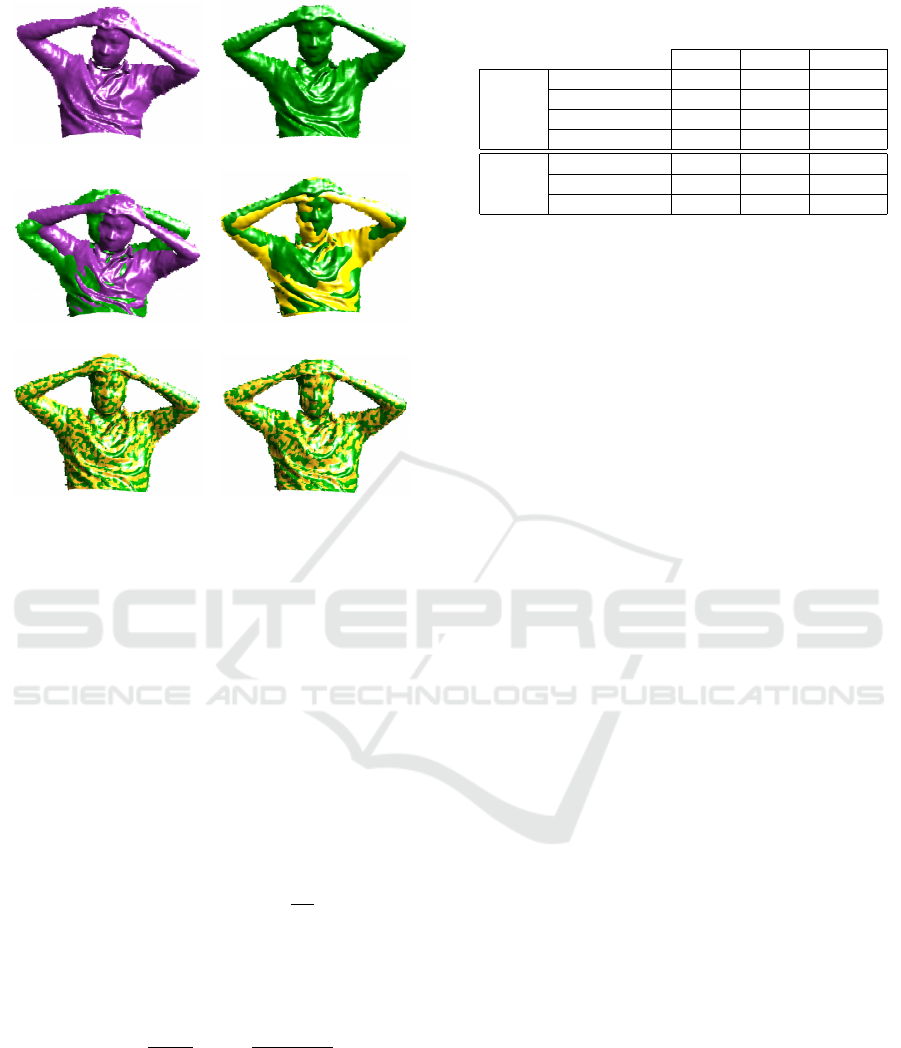
(a) (b)
(c) (d)
(e) (f)
Figure 3: Alignment results on low resolution data: (a)
source surface, (b) target surface, (c) before alignment, (d)
alignment result of GMM, (e) alignment result of TSA, (f)
our alignment result.
we set w
reg
= 10,w
f it
= 10. The optimization starts
with these values until convergence conditions are sat-
isfied:
E
n
− E
n−1
< 10
−7
or
z
n
− z
n−1
< 10
−6
.
Then, the value of w
reg
is reduced by half and the opti-
mization is initiated again. This procedure is repeated
until the value of w
reg
is less than 0.01. For each value
of w
reg
, the smoothing procedure is also applied for
corresponding points of nodes at each iteration:
E
s
( f ) =
m
∑
j=1
w
w
f(g
n
j
) −
¯
f(g
n
j
)
w
w
2
2
(11)
where f(g
n
j
) = u
j
− g
n
j
and
¯
f(g
n
j
) =
1
|C
j
|
∑
k∈C
j
f(g
n
k
) is
the mean of f over C
j
neighbors of u
j
(C
j
consists of
the points on the target surface in the sphere of radius
r
N
) and g
n
j
,g
n
k
are node positions at the n
th
iteration.
We also measure the distortion at each node:
M
d
=
1
N ( j)
∑
k∈N ( j)
|d
n
jk
− d
0
jk
|
d
0
jk
(12)
where d
0
jk
,d
n
jk
are distances between nodes before de-
formation and at iteration n. If M
d
is larger than
the threshold T
d
(in our experiments, T
d
= 0.2), the
node’s transformation is imposed only by the regular-
ization (Eq. 7).
Moreover, if a corresponding point lies on the
boundary of the target surface or the angle between
Table 1: Statistics for comparison between the GMM
method and our method.
Fig. 3 Fig. 4 Fig. 5
Ours
# points on S 69710 45942 113837
# points on T 70636 37761 113408
# nodes 1090 902 1016
Times(s) 452 307 487
GMM
# points on S 17353 11677 25519
# points on T 17590 9651 27461
Times(s) 2485 1476 5506
its normal and the node’s normal is greater than 45
degrees, the corresponding point is not used in the fit-
ting term at the current iteration.
4 EXPERIMENTAL RESULTS
Our method was implemented in MATLAB on a 3.2
GHz Intel Core i7 platform and its robustness was
compared with the method proposed in (Cao et al.,
2015) and another method (referred to as GMM in this
paper) proposed in (Jian and Vemuri, 2011). For the
implementation of GMM, its input data is obtained by
decimating the original size to 25% using the method
proposed in (Corsini et al., 2012). The statistics for
our method and GMM is shown in Table 1.
In the first experiment, shown in Fig. 3, we asked
a subject to sit in front of a Kinect camera. Be-
cause the camera provides low resolution data at each
frame, the data at each pose is obtained by merging
ten consecutive frames to collect more details. The
data at the second pose is a deformed version of that
at the first pose when the user twists the upper part of
his body. The data is presented in triangular meshes
and each mesh is comprised of a single patch. Us-
ing almost the same number of nodes for the defor-
mation graph in our method and TSA (1020 of TSA
and 1090 for ours), the optimization processes of the
two methods achieve optimal values to correctly align
the two surfaces (Fig. 3(e), 3(f)). Although the align-
ment result of TSA is slightly better than ours, our
method using a re-parameterized deformation model
is approximately four times faster (1658s of TSA and
452s for ours). GMM deforms the source surface
(second pose) by twisting this surface toward the tar-
get surface (first pose). However, when the head of
the source surface reaches that of the target surface,
the optimization process stops at a local minimum
and causes a misalignment between the two surfaces
(Fig. 3(d)). Moreover, the computation time of GMM
is five times higher than for our method although it
runs on a reduced-size data set.
The data in the next experiment was also acquired
by the Kinect camera (Fig. 4(a), 4(b)). In this exper-
GRAPP 2016 - International Conference on Computer Graphics Theory and Applications
44
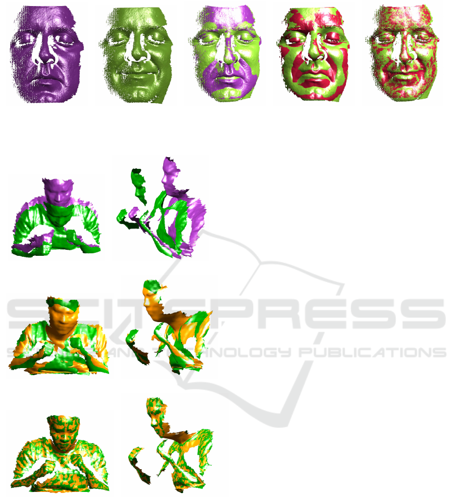
(a) (b) (c) (d) (e)
Figure 5: Alignment results between two surfaces of the disjointed connectivity: (a) source face, (b) target face, (c) before
alignment, (d) alignment result of GMM, (e) our result.
(a) (b)
(c) (d)
(e) (f)
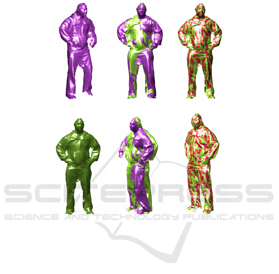
Figure 4: Alignment results for the data consisting of the
separated patches: face, torso, arms (view 1, view 2): (a, b)
before alignment, (c, d) alignment result of GMM, (e, f) our
alignment result.
iment, the surfaces consist of different patches due
to occlusion. In the TSA method, initial correspon-
dences and potential regions in the first stage are not
determined because the source surface (target surface)
cannot be used to generate a graph of the deformation
model (a sub-mesh), as shown in Fig. 2(b). TSA can-
not thus be applied in this case. GMM can be applied
because it is used to register two point sets. How-
ever, GMM also provides a misalignment in the fi-
nal result because the face is stretched and the left
arm is shrinked when the source surface deforms to-
ward the target surface (Fig. 4(c), 4(d)). In contrast,
our method creates a graph of 902 nodes and a sub-
mesh of 890 points and then aligns them together in
the first stage. Based on the results of this first stage,
in the second stage, the re-parameterized deformation
model is applied to obtain a good alignment between
the two surfaces (Fig. 4(e), 4(f)). As seen in the region
around the neck of the subject on the source surface,
our deformation process behaves elasticly as the neck
is elongated to align the two faces.
In the work of (Cao et al., 2015), the alignment be-
tween the two surfaces, which captures different ex-
pressions of a person’s face, is performed. It can be
used in applications such as 3D games, dynamic face
reconstruction or 3D face recognition. However, it is
required that the mesh of each surface be a continu-
ous mesh to create the sub-meshes. When one of the
two meshes is a disjoint mesh, as shown in Fig. 5(a),
5(b), this method cannot be applied. The deformation
between the two surfaces mostly occurs around the
mouth and cheek region. GMM deforms incorrectly
the mouth region of the source surface when align-
ing with one of the target surface (Fig. 5(d)). We ap-
ply our method and obtain the alignment result shown
in Fig. 5(e). Around the mouth rim, the source sur-
face does not align well with the target surface but
this issue can be solved by increasing the number of
nodes while allowing more time for the optimization
process to converge. From the experiments, we also
note that the computation time of GMM increases ex-
ponentially with the number of data points (Table 1)
while that of our method depends mainly on the num-
ber of nodes which can be specified by the user when
generating the graph of the deformation model.
In another comparison with TSA for aligning
small details between two surfaces, we register the
Re-parameterization of a Deformation Model for Non-rigid Registration
45
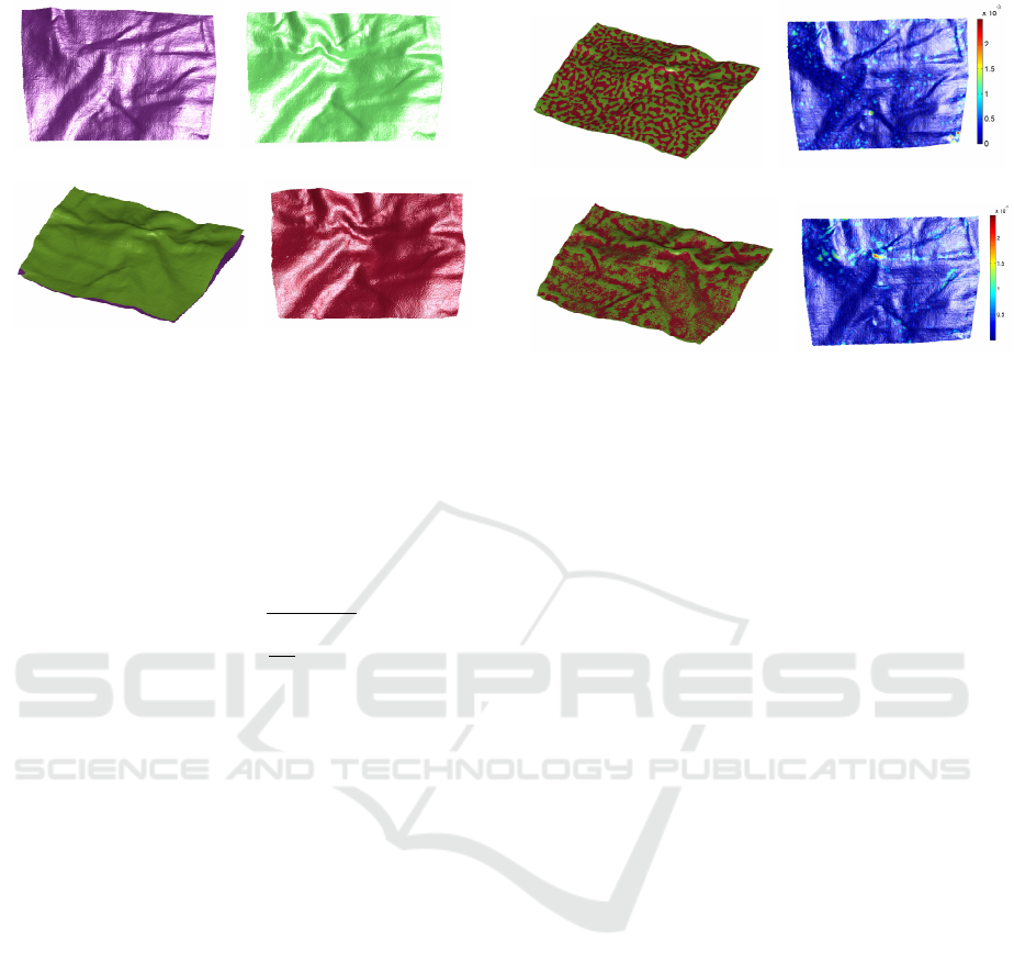
(a) (b)
(c) (d)
Figure 6: Our method deforms correctly to align small de-
tails on the pillow surfaces: (a) source surface, (b) tar-
get surface, (c) before alignment, (d) deformed version of
source surface.
two surfaces of a deformable pillow, as shown in
Fig. 6. This is high resolution data, the noise level
is low but the surfaces have many small creases. We
measure the root mean square error (RMS) based on
the squared distance function (Cao et al., 2015)
RMS(S,T ) =
v
u
u
t
1
|S|
|S|
∑
i=1
F
+
i
(13)
where |S| is the number of points on the source sur-
face and F
+
i
is value of squared distance function at
point
e
v
i
.
The deformed surface obtained with our method
is shown in Fig. 6(d) and the comparison with the
TSA method is shown in Fig. 7. In both methods, the
source surface is deformed to align correctly with the
target surface at small details (creases in this case).
Both methods use about 1000 nodes in the deforma-
tion graph, our RMS error (mm) is greater than that
of TSA (0.306 vs 0.164). However, this experiment
shows that our method can obtain a good alignment
with the presence of small details. We can accept a
slightly larger error while the alignment process can
be accelerated four times (597s vs 2212s).
In the last experiment, we register two high reso-
lution partial models which are acquired at the eighth
frame and the twenty-fourth frame by the system pro-
posed in (Vlasic et al., 2009). For this data, we use a
deformation graph with 1932 nodes and align it with
the target surface. As shown in Fig. 8, our method
with a re-parameterized deformation model is robust
and can align two models without any prior and as-
sumptions for non-rigid registration. This experiment
demonstrates that our method can be a promising so-
lution for 3D applications such as 3D dynamic recon-
struction, 3D animation or 3D retrieval for dynami-
(a) (b)
(c) (d)
Figure 7: Registration of pillow data: (a,b) alignment result
and error map of TSA, (c, d) alignment result and error map
of our method.
cally deformable objects.
5 CONCLUSION
In this paper, we present an improvement to a ro-
bust non-rigid registration method. The main con-
tribution of this work is to provide an alignment
method that can be applied to the data captured by
different types of 3D cameras with high frame rates
such as low or high resolution data, partial data, data
with small details and data under elastic deforma-
tion. The Euclidean distance is used in graph gener-
ation such that the method can be applied for meshes
with disconnected patches. We also develop a reg-
istration framework in a re-parameterized deforma-
tion model in which the computation time is reduced
and the optimization process is less complex. The
proposed method outperforms the GMM method in
alignment quality as well as computation time. Com-
pared with the TSA method, the alignment quality im-
plemented by the proposed method is almost as good
and achieves acceleration of around four times for the
alignment process. The presented method can be ap-
plied to different data types without any prior knowl-
edge of the geometry of the objects or assumptions.
ACKNOWLEDGMENTS
We are grateful to Myronenko and Song for pro-
viding us with the implementation of their method.
We would also like to thank Bonarrigo et al., Vla-
sic et al. for providing the 3D data sets. A special
thanks to Mrs. Annette Schwerdtfeger for proofread-
GRAPP 2016 - International Conference on Computer Graphics Theory and Applications
46
(a) (b) (c)
(d) (e) (f)
Figure 8: Our method is applied on the data of dynamic-deformable objects: (a) source surface, (d) target surface, (b, e) two
models before alignment (view 1, view 2), (c, f) our alignment results (view 1, view 2).
ing our manuscript. This research was supported by
the NSERC-Creaform Industrial Research Chair on
3D Scanning.
REFERENCES
Allen, B., Curless, B., and Popovi
´
c, Z. (2003). The space of
human body shapes: reconstruction and parameteriza-
tion from range scans. ACM Transactions on Graph-
ics, 22(3):587–594.
Amberg, B., Romdhani, S., and Vetter, T. (2007). Optimal
step nonrigid icp algorithms for surface registration.
In Computer Vision and Pattern Recognition, 2007.
CVPR ’07. IEEE Conference on, pages 1–8.
Anguelov, D., Srinivasan, P., Pang, H., Koller, D., Thrun,
S., and Davis, J. (2004). The correlated correspon-
dence algorithm for unsupervised registration of non-
rigid surfaces. In Advances in Neural Information
Processing Systems 17 [Neural Information Process-
ing Systems, NIPS 2004, December 13-18, 2004, Van-
couver, British Columbia, Canada], pages 33–40.
Bernardini, F., Mittleman, J., Rushmeier, H., Silva, C., and
Taubin, G. (1999). The ball-pivoting algorithm for
surface reconstruction. IEEE Transactions on Visual-
ization and Computer Graphics, 5(4):349–359.
Bonarrigo, F., Signoroni, A., and Botsch, M. (2014). De-
formable registration using patch-wise shape match-
ing. Graphical Models, 76(5):554 – 565. Geometric
Modeling and Processing 2014.
Cao, V., Nguyen, V., Tran, T., Ali, S., and Laurendeau, D.
(2014). Non-rigid registration for deformable objects.
In GRAPP 2014 - Proceedings of the 9th International
Conference on Computer Graphics Theory and Appli-
cations, Lisbon, Portugal, 5-8 January, 2014., pages
43–52.
Cao, V.-T., Tran, T.-T., and Laurendeau, D. (2015). A two-
stage approach to align two surfaces of deformable
objects. Graphical Models, 82:13 – 28.
Chang, W. and Zwicker, M. (2008). Automatic registration
for articulated shapes. In Proceedings of the Sympo-
sium on Geometry Processing, SGP ’08, pages 1459–
1468, Aire-la-Ville, Switzerland. Eurographics Asso-
ciation.
Re-parameterization of a Deformation Model for Non-rigid Registration
47

Chen, S.-G. and Wu, J.-Y. (2004). Estimating normal vec-
tors and curvatures by centroid weights. Computer
Aided Geometric Design, 21(5):447 – 458.
Corsini, M., Cignoni, P., and Scopigno, R. (2012). Efficient
and flexible sampling with blue noise properties of tri-
angular meshes. IEEE Transactions on Visualization
and Computer Graphics, 18(6):914–924.
Dou, M., Taylor, J., Fuchs, H., Fitzgibbon, A., and Izadi, S.
(2015). 3d scanning deformable objects with a single
rgbd sensor. In The IEEE Conference on Computer
Vision and Pattern Recognition (CVPR).
Grassia, F. S. (1998). Practical parameterization of rotations
using the exponential map. Journal of Graphics Tools,
3(3):29–48.
Huang, Q.-X., Adams, B., Wicke, M., and Guibas, L. J.
(2008). Non-rigid registration under isometric defor-
mations. In Proceedings of the Symposium on Geom-
etry Processing, SGP ’08, pages 1449–1457, Aire-la-
Ville, Switzerland. Eurographics Association.
Jian, B. and Vemuri, B. (2011). Robust point set registra-
tion using gaussian mixture models. Pattern Analy-
sis and Machine Intelligence, IEEE Transactions on,
33(8):1633–1645.
Li, H., Adams, B., Guibas, L. J., and Pauly, M. (2009). Ro-
bust single-view geometry and motion reconstruction.
ACM Transactions on Graphics, 28(5):175:1–175:10.
Li, H., Sumner, R. W., and Pauly, M. (2008). Global cor-
respondence optimization for non-rigid registration of
depth scans. In Proceedings of the Symposium on Ge-
ometry Processing, SGP ’08, pages 1421–1430, Aire-
la-Ville, Switzerland. Eurographics Association.
Li, H., Vouga, E., Gudym, A., Luo, L., Barron, J. T., and
Gusev, G. (2013). 3d self-portraits. ACM Transactions
on Graphics, 32(6):1–9.
Myronenko, A. and Song, X. (2010). Point set registration:
Coherent point drift. Pattern Analysis and Machine
Intelligence, IEEE Transactions on, 32(12):2262–
2275.
Newcombe, R. A., Fox, D., and Seitz, S. M. (2015). Dy-
namicfusion: Reconstruction and tracking of non-
rigid scenes in real-time. In The IEEE Conference on
Computer Vision and Pattern Recognition (CVPR).
Peyr
´
e, G. and Cohen, L. D. (2006). Geodesic remeshing us-
ing front propagation. International Journal of Com-
puter Vision, 69(1):145–156.
Rouhani, M., Boyer, E., and Sappa, A. D. (2014). Non-
rigid registration meets surface reconstruction. In 3D
Vision (3DV), 2014 2nd International Conference on,
volume 2, pages 617–624.
Sagawa, R., Akasaka, K., Yagi, Y., Hamer, H., and
Van Gool, L. (2009). Elastic convolved icp for the
registration of deformable objects. In Computer Vi-
sion Workshops (ICCV Workshops), 2009 IEEE 12th
International Conference on, pages 1558–1565.
Schmidt, J. and Niemann, H. (2001). Using quaternions for
parametrizing 3-d rotations in unconstrained nonlin-
ear optimization. In Vision, Modeling, and Visualiza-
tion 2001, pages 399–406. AKA/IOS Press.
Sumner, R. W., Schmid, J., and Pauly, M. (2007). Embed-
ded deformation for shape manipulation. ACM Trans-
actions on Graphics, 26(3).
Terzakis, G., Culverhouse, P., Bugmann, G., Sharma, S.,
and Sutton, R. (2012). A recipe on the parameter-
ization of rotation matrices for non-linear optimiza-
tion using quaternions. Technical report, Center for
Robotics and Neural Systems, Plymouth University,
Plymouth, UK.
Vlasic, D., Peers, P., Baran, I., Debevec, P., Popovi
´
c, J.,
Rusinkiewicz, S., and Matusik, W. (2009). Dynamic
shape capture using multi-view photometric stereo.
ACM Transactions on Graphics, 28(5):174:1–174:11.
Zeng, M., Zheng, J., Cheng, X., and Liu, X. (2013).
Templateless quasi-rigid shape modeling with implicit
loop-closure. In Computer Vision and Pattern Recog-
nition (CVPR), 2013 IEEE Conference on, pages 145–
152.
Zhang, L., Snavely, N., Curless, B., and Seitz, S. M. (2004).
Spacetime faces: High resolution capture for model-
ing and animation. ACM Transactions on Graphics,
23(3):548–558.
Zhang, Q., Fu, B., Ye, M., and Yang, R. (2014). Quality dy-
namic human body modeling using a single low-cost
depth camera. In Computer Vision and Pattern Recog-
nition (CVPR), 2014 IEEE Conference on, pages 676–
683.
Zhang, R., Chen, X., Shiratori, T., Tong, X., and Liu, L.
(2015). An efficient volumetric method for non-rigid
registration. Graphical Models, 79:1 – 11.
Zollh
¨
ofer, M., Nießner, M., Izadi, S., Rehmann, C., Zach,
C., Fisher, M., Wu, C., Fitzgibbon, A., Loop, C.,
Theobalt, C., and Stamminger, M. (2014). Real-time
non-rigid reconstruction using an rgb-d camera. ACM
Transactions on Graphics, 33(4):156:1–156:12.
APPENDIX
In iterative non-linear optimization process of our
method, calculation of Jacobian matrix plays an im-
portant role for correctly updating the parameters at
each iteration. This process relates to computing the
derivatives of each rotation matrix R
j
with respect to
a given value (x
j
,y
j
,z
j
) of a point ψ
j
on the equatorial
plane.
The derivatives of a rotation matrix R with respect
to a point ψ are calculated using the chain rule as fol-
lows (for simplicity, we remove the index j ):
∂R(q(ψ))
∂x
=
3
∑
n=0
∂R(q)
∂q
n
∂q
n
(ψ)
∂x
(14)
∂R(q(ψ))
∂y
=
3
∑
n=0
∂R(q)
∂q
n
∂q
n
(ψ)
∂y
(15)
∂R(q(ψ))
∂z
=
3
∑
n=0
∂R(q)
∂q
n
∂q
n
(ψ)
∂z
(16)
A rotation matrix parameterized by a unit-
quaternion is given by the following formula:
GRAPP 2016 - International Conference on Computer Graphics Theory and Applications
48

R(q) =
q
2
0
+ q
2
1
− q
2
2
− q
2
3
2(q
1
q
2
− q
0
q
3
) 2(q
1
q
3
+ q
0
q
2
)
2(q
1
q
2
+ q
0
q
3
) q
2
0
− q
2
1
+ q
2
2
− q
2
3
2(q
2
q
3
− q
0
q
1
)
2(q
1
q
3
− q
0
q
2
) 2(q
2
q
3
+ q
0
q
1
) q
2
0
− q
2
1
− q
2
2
+ q
2
3
(17)
The partial derivatives of the rotation matrix with
respect to the unit-quaternion are:
∂R(q)
∂q
0
= 2
q
0
−q
3
q
2
q
3
q
0
−q
1
−q
2
q
1
q
0
(18)
∂R(q)
∂q
1
= 2
q
1
q
2
q
3
q
2
−q
1
−q
0
q
3
q
0
−q
1
(19)
∂R(q)
∂q
2
= 2
−q
2
q
1
q
0
q
1
q
2
q
3
−q
0
q
3
−q
2
(20)
∂R(q)
∂q
3
= 2
−q
3
−q
0
q
1
q
0
−q
3
q
2
q
1
q
2
q
3
(21)
The partial derivatives of unit quaternion with re-
spect to the point ψ = (x,y,z) are:
∂q(ψ)
∂x
=
2
1+α
2
−
4x
2
(1+α
2
)
2
−
4xy
(1+α
2
)
2
−
4xz
(1+α
2
)
2
−
4x
(1+α
2
)
2
(22)
∂q(ψ)
∂y
=
−
4xy
(1+α
2
)
2
2
1+α
2
−
4y
2
(1+α
2
)
2
−
4yz
(1+α
2
)
2
−
4y
(1+α
2
)
2
(23)
∂q(ψ)
∂z
=
−
4xz
(1+α
2
)
2
−
4yz
(1+α
2
)
2
2
1+α
2
−
4z
2
(1+α
2
)
2
−
4z
(1+α
2
)
2
(24)
Re-parameterization of a Deformation Model for Non-rigid Registration
49
