Adaptive Two-stage Learning Algorithm for Repeated Games

Wataru Fujita

, Koichi Moriyama

, Ken-ichi Fukui

1,3

and Masayuki Numao

1,3

Graduate School of Information Science and Technology, Osaka University,

1-5, Yamadaoka, Suita, Osaka, 565-0871, Japan

Graduate School of Engineering, Nagoya Institute of Technology, Gokiso-cho, Showa-ku, Nagoya, 466-8555, Japan

The Institute of Scientiﬁc and Industrial Research, Osaka University, 8-1, Mihogaoka, Ibaraki, Osaka, 567-0047, Japan

Keywords:

Multi-agent, Reinforcement Learning, Game Theory.

Abstract:

In our society, people engage in a variety of interactions. To analyze such interactions, we consider these

interactions as a game and people as agents equipped with reinforcement learning algorithms. Reinforcement

learning algorithms are widely studied with a goal of identifying strategies of gaining large payoffs in games;

however, existing algorithms learn slowly because they require a large number of interactions. In this work,

we constructed an algorithm that both learns quickly and maximizes payoffs in various repeated games. Our

proposed algorithm combines two different algorithms that are used in the early and later stages of our algo-

rithm. We conducted experiments in which our proposed agents played ten kinds of games in self-play and

with other agents. Results showed that our proposed algorithm learned more quickly than existing algorithms

and gained sufﬁciently large payoffs in nine games.

1 INTRODUCTION

Humans make a variety of decisions in their daily

lives. In social situations in which a person’s deci-

sion depends on other people, there are complicated

mutual relations such as competition and cooperation

among people. Many researchers have widely stud-

ied game theory that models relations among people

as “games” and analyzed rational decision-making in

games.

Furthermore, humans have an instinctive desire

for survival; therefore, learning through trial-and-

error to avoid harmful and unpleasant states and ap-

proach beneﬁcial and pleasant states. Such learn-

ing occurs given a learning mechanism in the human

brain. Many researchers study reinforcement learning

algorithms that model this learning mechanism.

Let us consider people who learn their behavior

from the result of interacting with others. As a model

of this, we discuss reinforcement learning agents that

play games. Many (multi-agent) reinforcement learn-

ing algorithms that perform well in various games

have already been proposed; however, such algo-

rithms typically require a large number of interactions

to learn appropriate behavior in the games. People in

the real world must quickly learn to make reasonable

decisions, because the world changes rapidly. Exist-

ing algorithms have various features, each with its ad-

vantages and disadvantages. These algorithms can be

complementary. Therefore, in this study, we construct

an algorithm that learns quickly and performs well in

any type of game by combining features from multi-

ple algorithms.

Aside from this introductory section, the structure

of this paper is as follows. In Section 2, we intro-

duce games and learning algorithms used in later sec-

tions. In Section 3, we construct a new learning algo-

rithm that learns quickly and performs well in various

games by combining two learning algorithms. Next,

we evaluate our proposed algorithm by conducting

experiments, as described in Section 4. In Section 5,

we introduce related works to show the relative posi-

tion of our algorithm. Finally, in Section 6, we con-

clude our paper and provide avenues for future work.

2 BACKGROUND

In this section, we introduce game theory that models

interactions among people and reinforcement learn-

ing algorithms that model trial-and-error learning for

adaptation to a given environment.

Fujita, W., Moriyama, K., Fukui, K-i. and Numao, M.

Adaptive Two-stage Learning Algorithm for Repeated Games.

DOI: 10.5220/0005711000470055

In Proceedings of the 8th International Conference on Agents and Artiﬁcial Intelligence (ICAART 2016) - Volume 1, pages 47-55

ISBN: 978-989-758-172-4

2.1 Game Theory

We, as humans, are always making decisions as to

what to do next to achieve our desired purpose or

goals. In social environments, every decision is af-

fected by the decisions of other people. Game theory

(Okada, 2011) mathematically analyzes the relation-

ship among such decisions.

A game in game theory consists of the following

four elements (Okada, 2011):

1. Rules that govern the game;

2. Players who decide what to do;

3. Action strategies of the players; and

4. Payoffs given to the players as a result of their

decisions.

Game theory analyzes how players behave in an

environment in which their actions mutually inﬂuence

one another. We focus on two-person simultaneous

games in this study.

In a two-person simultaneous game, two players

simultaneously choose actions based on their given

strategies. After both players choose their respective

actions, each player is given a payoff determined by

the “joint actions” of both players. Since the payoff of

each player is determined by not only his or her action

but also the other player’s action, it is necessary to de-

liberate the other player’s action to maximize payoffs.

Note that all games used in this research are non-

cooperative game, and players choose their individual

strategies based on its own payoffs and all players’

actions. More speciﬁcally, after a player observes its

payoffs and the action of the other players, he or she

can then choose his or her own self-strategy.

A Nash equilibrium is deﬁned as the combination

of actions in which no player is motivated to change

his or her strategy. Let us consider the ”prisoner’s

dilemma” game summarized in Table 1. Here, the row

and column correspond to the actions of Players 1 and

2, respectively; they gain the left and right payoffs,

respectively, corresponding to the joint action in the

matrix.

According to the payoff matrix, the player should

choose the Defection action regardless of the other

player’s action, because it always yields higher pay-

offs than the Cooperation action. Since the other

player considers the same, both players choose De-

fection, and ﬁnally, the combination of actions (i.e.,

Defection, Defection) becomes a Nash equilibrium.

Conversely, if both players select Cooperation,

both payoffs can be raised to 0.6 from 0.2; however,

it is very difﬁcult for both players to choose Coopera-

tion, because the combination (i.e., Cooperation, Co-

operation) does not yield equilibrium and each player

is motivated to choose Defection. Moreover, even if a

player overcomes this motive for a certain reason, he

or she will yield a payoffof zero if the partner chooses

Defection. The prisoner’s dilemma game shows that

the individual’s rationality differs from that of social

rationality in a social situation.

Table 1: An example of payoffs in the prisoner’s dilemma

game.

Cooperation Defection

Cooperation 0.6,0.6 0.0,1.0

Defection 1.0,0.0 0.2,0.2

2.2 Reinforcement Learning

Reinforcement learning (Sutton and Barto, 1998) is a

learning method that learns strategies by interacting

with the given environment. An agent is deﬁned as a

decision-making entity, while the environment is ev-

erything external to the agent that interacts with the

agent. Furthermore, the agent interacts with the en-

vironment at discrete time steps, i.e., t = 0,1,2,3,....

At each time step t, the agent recognizes current state

∈ S of the environment, where S is a set of possible

states, and decides action a

∈ A(s

) based on the cur-

rent state, where A(s

) is a set of actions selectable in

state s

At the next step, the agent receives reward r

t+1

∈

ℜ as a result of the action and transitions to new state

t+1

. The probability that the agent chooses possible

action a in state s is shown as strategy π

(s,a). Re-

inforcement learning algorithms update strategy π

the action values (not the strategy) at each time step,

choosing an action based on the strategy.

2.3 Three Foundational Learning

Algorithms

Here we introduce three learning algorithms that form

the basis for our proposal.

2.3.1 M-Qubed

M-Qubed (Crandall and Goodrich, 2011) is an excel-

lent state-of-the-art reinforcement learning algorithm

that consists of three strategies that can learn to coop-

erate with associates (i.e., other players) and avoid be-

ing exploited unilaterally in various games. M-Qubed

uses Sarsa (Rummery and Niranjan, 1994) to learn ac-

tion value function Q(s,a) (called the Q-value), which

means the value of action a in state s. Here, state is

deﬁned as the latest joint action of the agent and its as-

sociates. Further, Q(s,a) is updated by the following

ICAART 2016 - 8th International Conference on Agents and Artiﬁcial Intelligence

rule:

t+1

)

= Q

) + α[r

+ γV

t+1

) − Q

)],

(1)

(s) =

∑

a∈A(s)

(s,a)Q

(s,a), (2)

where r

t+1

∈ [0, 1], α is the learning rate, and γ is the

discount rate.

After M-Qubed updates the Q-value, it calculates

the strategy of the agent from three sub-strategies,

i.e., “Proﬁt pursuit”, “Loss aversion”, or “Optimistic

search”. Each of these is described below. Further,

the maximin value is the secured payoff regardless

of the associates given by the maximin strategy that

maximizes the minimum payoff based on the payoff

deﬁnition of the game.

Proﬁt Pursuit

This sub-strategy takes the action with the max-

imum Q-value if it is larger than the discounted

sum of the maximin value; otherwise, the max-

imin strategy is used.

Loss Aversion

This sub-strategy takes the action with the maxi-

mum Q-value if the accumulated loss is less than

a given threshold; otherwise, the maximin strat-

egy is used. Here, the accumulated loss is the dif-

ference between the accumulated payoffs and the

accumulated maximin value. The threshold is set

proportional to the number of possible states and

joint actions.

Optimistic Search

The “Proﬁt pursuit” strategy can acquire high pay-

offs for the moment; however, it tends to produce

myopic actions as a result. The “Loss aversion”

strategy cannot lead cooperative strategies with

associates, which may yield higher payoffs. To

solve these problems, M-Qubed sets the initial Q-

values to their highest possible discounted reward

1/(1− γ), thereby learning wider strategies.

Next, the strategy is a weighted average of “Proﬁt

pursuit” and “Loss aversion”, and Q-values are ini-

tialized by “Optimistic search”.

However, if all recently visited states have low Q-

values, the strategies of the agent and its associates

may remain at a local optimum. The agent must ex-

plore further to ﬁnd a solution that may give a higher

payoff. Hence, in this case, the strategy is changed to

a weighted average of the above strategy and a com-

pletely random strategy.

2.3.2 Satisﬁcing Algorithm

Satisﬁcing algorithm (S-alg) (Stimpson and

Goodrich, 2003) is an algorithm that calculates

a value called the aspiration level of the agent. The

agent continues to take an action that gives payoffs

more than its aspiration level. The algorithm is shown

in Algorithm 1.

Algorithm 1: Satisﬁcing algorithm.

Parameters:

t: time

: aspiration level at time t

: my action at time t

: payoff at time t

λ ∈ (0, 1): learning rate

Initialize:

t = 0

Set α

randomly between the maximum payoff

max

and 2R

max

repeat

Select a

if r

t−1

≥ α

t−1

then

← a

t−1

else if otherwise then

← Random

end if

Receive r

and update α

t+1

← λα

+ (1− λ)r

t ← t + 1

until Game Over

S-alg is an algorithm that enables an agent to learn

to take cooperative actions with its associates.

2.3.3 BM Algorithm

Fujita et al. (2016) proposed BM algorithm to maxi-

mize payoffs by combining M-Qubed and S-alg. BM

algorithm comprises the above two learning algo-

rithms and creates a new strategy that combines the

strategies derived from the two internal algorithms.

Both algorithms simultaneously update their func-

tions, i.e., the Q-value and aspiration level.

BM algorithm uses a Boltzmann multiplication

(Wiering and van Hasselt, 2008) as the method of

combination. Based on strategy π

of internal algo-

rithm j, Boltzmann multiplication multiplies strate-

gies of all internal algorithms for each available action

and determines the ensemble strategy by the Boltz-

mann distribution. The preference values of actions

are deﬁned as

,a[i]) =

∏

,a[i]) (3)

Adaptive Two-stage Learning Algorithm for Repeated Games

and the resulting ensemble strategy is deﬁned as

,a[i]) =

,a[i])

∑

,a[k])

, (4)

where a[i] is a possible action and τ is a temperature

parameter. After calculating the ensemble strategy,

the agent selects an action, and then all internal algo-

rithms learn from the result of this selected action.

Since S-alg yields only pure strategies, all actions

except for the chosen one have zero probability. The

M-Qubed becomes meaningless when the Boltzmann

multiplication is used to combine M-Qubed and S-alg

without consideration. Therefore, the S-alg in BM

algorithm yields a mixed strategy in which the chosen

action is played with probability 0.99.

3 PROPOSED ALGORITHM

In this study, we consider reinforcement learning

agents that play games. M-Qubed, BM, and S-alg

agents perform well in some games, but have prob-

lems in other games, as summarized below:

• M-Qubed requires a long time to learn, because it

has multiple strategies and needs to decide which

one is used. Therefore, the average payoff be-

comes less than S-alg in the game having only one

suitable solution that is in cooperation with the as-

sociates.

• BM algorithm performs better than M-Qubed, but

it is still slow in search because the internal S-alg

cannot completely compensate for the slowness of

M-Qubed.

• If the associates are greedy, S-alg is exploited uni-

laterally, because it decreases the aspiration level,

and then S-alg is satisﬁed with low payoffs.

• Due to insufﬁcient search, S-alg may be satisﬁed

with the second-best payoff.

These algorithms do not have sufﬁcient perfor-

mance for a variety of reasons; however, their posi-

tive abilities are complementary. BM, which is not

exploited due to the “Loss aversion” strategy and ex-

plores the given environment thoroughly enough, can

compensate for the weakness of S-alg that tends to be

exploited. Conversely, S-alg, which quickly learns to

cooperate, can compensate for the weakness of BM,

i.e., its slowness of search. Search in an early stage

of interactions and the secured payoff are important

when the agent learns. Therefore, we combine BM

and S-alg to construct an algorithm that quickly learns

good strategies in various games.

We call our proposed algorithm J-algorithm (J-

alg). J-alg has an Exploration stage and a Static stage.

The Exploration stage is represented by our S’ algo-

rithm, which is a slightly modiﬁed version of S-alg.

Similarly, the Static stage is represented by BM algo-

rithm. In the following subsections, we introduce our

S’ algorithm (i.e., S’-alg) and our proposed two-stage

J-alg.

3.1 S’ Algorithm

We focused on S-alg to play a key role in the Ex-

ploration stage, because S-alg can learn to cooperate

quickly; however, S-alg tends to cover an insufﬁcient

search space and falls prey to a myopic strategy. Sup-

pose that the S-alg agents play the Security game (SG)

shown in Table 2. If the aspiration level of the row

player is smaller than 0.84, the player loses his or her

motivation to change his or her action from x. Con-

sequently, both players are satisﬁed with a payoff that

is not the largest one. S-alg stops searching for other

actions and is therefore prone to a shortened search.

Table 2: Security game (SG).

z w

x 0.84, 0.33 0.84, 1.0

y 0.0, 1.0 1.0, 0.67

To solve this problem, we slightly modify S-alg

to add new action b; this new algorithm is called the

S’ algorithm (i.e., S’-alg). In short, in S’-alg, if the

agent receives the maximin value as the last payoff, it

selects action b. The modiﬁed algorithm is shown in

Algorithm 2.

This change stochastically forces the agent to take

other actions to escape from a local solution and po-

tentially ﬁnd a better one.

3.2 Integrating the Two Stages

J-alg uses S’-alg for the Exploration stage and BM for

the Static stage. The J-alg agent starts in the Explo-

ration stage. After the joint action converges, the al-

gorithm switches to the Static stage and resets the Q-

values to choose the converged action more often. If

the joint action does not convergein the ﬁrst t

rounds,

the algorithm simply changes to the Static stage with-

out changing the value. The algorithm is shown in

Algorithm 3.

Even though the J-alg agent is exploited in the

Exploration stage, it will recover in the Static stage

via BM algorithm that can evade a loss by using

“Loss aversion” strategy.

ICAART 2016 - 8th International Conference on Agents and Artiﬁcial Intelligence

Algorithm 2: S’ algorithm.

Parameters:

t: time

: aspiration level at time t

: my action at time t

: payoff at time t

λ ∈ (0, 1): learning rate

b: a random action other than a

t−1

with probabil-

ity p and a random action selected from all of the

actions with probability (1− p)

Initialize:

t = 0

Set α

randomly between the maximum payoff

max

and 2R

max

repeat

Select a

if r

t−1

≥ α

t−1

then

← a

t−1

else if r

t−1

= maximin value then

← b

else if otherwise then

← Random

end if

Receive r

and update α

t+1

← λα

+ (1− λ)r

t ← t + 1

until Game Over

4 EXPERIMENTS

To conﬁrm sufﬁcient performance of J-alg, we con-

ducted experiments using 10 two-person two-action

matrix games used in the M-Qubed paper (Crandall

and Goodrich, 2011). Here, the agent can observe

only the previous joint action and its own payoff. We

also set the M-Qubed parameters to be identical to the

original ones noted in Crandall and Goodrich (2011).

We set parameter τ of the BM algorithm to 0.2. Fur-

ther, we set learning rate λ = 0.99, probability p = 0.3

of S’-alg, reduction rate δ = 0.99 and time t

= 500

for the threshold at which a shift occurs from the Ex-

ploration stage to the Static stage. We considered that

a certain joint action converged when it had contin-

ued 30 rounds. Table 3 shows the games used in our

experiments. Here, we call the maximum joint action

a joint action by which the sum of both player’s pay-

offs becomes maximum (which is shown in bold italic

typeface in the table).

4.1 Experiment 1

Our ﬁrst experiment was conducted in games

where both players are agents with the same algo-

Algorithm 3: J-alg.

Parameters:

s: state

a: action

: my action when joint action converges

: payoff when joint action converges

δ ∈ [0, 1]: reduction rate

Initialize:

t = 1

Start the Exploration stage

repeat

if in the Exploration stage and t < t

then

if joint action has not converged then

Continue the Exploration stage

else if otherwise then

if a = a

then

Q(s,a) ← r

/(1− γ)

else if otherwise then

Q(s,a) ← δ × r

/(1− γ)

for all s.

Start the Static stage

end if

else if otherwise then

Start the Static stage

end if

t ← t + 1

until Game Over

rithm, i.e., in self-play. Agents played one of the 10

games for 50000 rounds, iterating 50 times for each

game. We then compared the normalized average

payoffs of M-Qubed, S-alg, BM, and J-alg. Note that

the earlier the actions of agents converge to the max-

imum joint action, the larger the normalized average

payoffs become. Table 4 shows the normalized aver-

age payoffs in the games, each of which is the average

payoff divided by that of the maximum joint action. If

the normalized averagepayoffis close to one, it shows

that the agent quickly learned the maximum joint ac-

tion in the game.

From our results, we observe that J-alg gained

high payoffs and quickly learned the maximum joint

action of nine games in self-play. It was able to learn

optimal strategies more quickly than M-Qubed and

BM due to the Exploration stage (i.e., S’-alg). M-

Qubed and BM particularly gained low payoffs in the

prisoner’s dilemma (PD) game, because of the mutual

defection (b,d) by performing many explorations to

learn the cooperative joint action (a,c). S-alg gained

high payoffs in eight games, not including the secu-

rity game (SG) and the offset game (OG). In these

games, the aspiration level of S-alg decreased be-

low the second-best payoff because of insufﬁcient ex-

Adaptive Two-stage Learning Algorithm for Repeated Games

Table 3: Payoff matrices of the two-person two-action ma-

trix games used in our experiments. The row player has two

actions, a and b, and the column player has two actions, c

and d. The values in the cells show the payoffs the play-

ers are given when the joint action appears (i.e., left for the

row player and right for the column player). Payoffs in bold

italic typeface are those that maximize the sum of the two

payoffs.

(a) Common interest game (CIG)

c d

a 1.0, 1.0 0.0, 0.0

b 0.0, 0.0 0.5, 0.5

(b) Coordination game (CG)

c d

a 1.0, 0.5 0.0, 0.0

b 0.0, 0.0 0.5, 1.0

c d

a 1.0, 1.0 0.0, 0.75

b 0.75, 0.0 0.5, 0.5

(d) Tricky game (TG)

c d

a 0.0, 1.0 1.0, 0.67

b 0.33, 0.0 0.67, 0.33

(e) Prisoner’s dilemma (PD)

c d

a 0.6, 0.6 0.0, 1.0

b 1.0, 0.0 0.2, 0.2

(f) Battle of the sexes (BS)

c d

a 0.0, 0.0 0.67, 1.0

b 1.0, 0.67 0.33, 0.33

(g) Chicken (Ch)

c d

a 0.84, 0.84 0.33, 1.0

b 1.0, 0.33 0.0, 0.0

(h) Security game (SG)

c d

a 0.84, 0.33 0.84, 0.0

b 0.0, 1.0 1.0, 0.67

(i) Offset game (OG)

c d

a 0.0, 0.0 0.0, 1.0

b 1.0, 0.0 0.0, 0.0

(j) Matching pennies (MP)

c d

a 1.0, 0.0 0.0, 1.0

b 0.0, 1.0 1.0, 0.0

Table 4: Normalized average payoffs when agents played

games in self-play. The bold typeface indicates the best re-

sults among the four given methods.

J-alg M-Qubed S-alg BM

CIG 0.999080 0.993804 0.999039 0.999181

CG 0.951450 0.847301 0.997966 0.867965

SH 0.999182 0.995857 0.999149 0.998505

TG 0.998033 0.814068 0.998251 0.828770

PD 0.998569 0.711794 0.998626 0.723831

BS 0.998686 0.910656 0.998700 0.917655

Ch 0.998909 0.934089 0.998900 0.931541

SG 0.998612 0.902031 0.718236 0.907887

OG 0.466739 0.473539 0.499964 0.478196

MP 1.000000 1.000000 1.000000 1.000000

Avg. 0.940926 0.858314 0.920883 0.865353

ploration. For all algorithms, the offset game (OG)

proved difﬁcult to learn the optimal strategy.

4.2 Experiment 2

In our second experiment, we compared J-alg with

M-Qubed, S-alg, and BM in round-robin tournaments

in which all combinations of agents were examined.

As with Experiment 1, the agents played one of the

10 games 50000 times, iterating 50 times for each

game. In asymmetric games, we replaced the posi-

tion of players and started our experiment again. The

normalized average payoffs of each game are shown

in Table 5. Values greater than one indicate that the

agent exploited other agents and gained high payoffs

as a result. If the average value of the normalized

average payoffs became larger, the agent gained high

payoffs across many rounds.

Table 5: Normalized average payoffs when agents play

games in round-robin tournaments. The bold typeface in-

dicates the best results from among the four given methods.

J-alg M-Qubed S-alg BM

CIG 0.998983 0.995743 0.998991 0.998603

CG 1.048619 0.915732 0.832476 0.905246

SH 0.999098 0.996896 0.999148 0.998226

TG 0.952595 0.863191 0.943683 0.868901

PD 0.900618 0.743598 0.871854 0.754596

BS 0.988460 1.002762 0.921269 0.951607

Ch 0.974938 0.933062 0.975377 0.926621

SG 0.935857 0.881564 0.810752 0.885159

OG 0.555748 0.497452 0.341784 0.538482

MP 1.041080 1.051359 0.858698 1.048864

Avg. 0.939600 0.888136 0.855403 0.887630

J-alg gained high average payoffs in many of the

games we used for our experiments. In the coordi-

nation game (CG), battle of the sexes (BS), the secu-

rity game (SG), the offset game (OG), and matching

pennies (MP), S-alg was exploited when the associate

took a greedy strategy, because its aspiration level de-

creased too much, and as a result, it was satisﬁed with

small payoffs. M-Qubed and BM were not able to

learn optimal strategies quickly and gain high aver-

age payoffs because they required a large number of

interactions. Note that M-Qubed did indeed gain high

average payoffs in battle of the sexes (BS) and match-

ing pennies (MP) by taking a greedy strategy.

The average payoffs shown in Table 4 and Ta-

ble 5 show that J-alg gained the highest average pay-

offs both in self-play and round-robin tournaments.

S-alg gained high payoffs in self-play, but it was ex-

ploited by greedy players and gained low payoffs in

round-robin tournaments. M-Qubed and BM gained

better payoffs by exploiting S-alg in round-robin tour-

naments than in self-play. However, they required a

large number of rounds to learn the maximum joint

action and therefore gained lower average payoffs

than that of J-alg.

4.3 Experiment 3

In our third experiment, we investigated whether S’-

alg actually contributed to the learning speed of J-alg.

Figure 1 shows learning curves of J-alg, M-Qubed,

S-alg, and BM in the common interest game (CIG),

stag hunt (SH), and the security game (SG). Results

of these three games are good examples that show

ICAART 2016 - 8th International Conference on Agents and Artiﬁcial Intelligence















         









(a) Common Interest Game (CIG)















               









(b) Stag Hunt (SH)















    









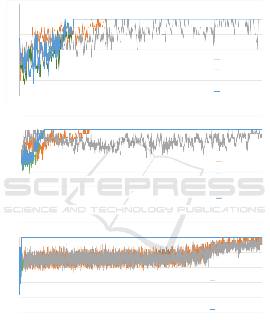
Figure 1: Learning curves of the four algorithms in self-play in three games. Blue lines show the curves of J-alg, gray show

those of M-Qubed, orange show those of BM, and green show those of S-alg. The x-axes show the rounds the agents played,

while the y-axes show normalized average payoffs.

how the algorithms comprised in J-alg complement

one another.

Figure 1(a), i.e., results of the common inter-

est game (CIG), shows that J-alg and S-alg quickly

Adaptive Two-stage Learning Algorithm for Repeated Games

learned the maximum joint action almost simultane-

ously. BM learned the maximum joint action by the

190th round, shortly after J-alg and S-alg. M-Qubed

was still learning at the 500th round. Results here

show that S’-alg contributed to the learning speed of

J-alg.

Results of the stag hunt (SH) game are shown in

Fig. 1(b), which shows that J-alg and S-alg ﬁnished

learning the maximum joint action the quickest. Next,

BM ﬁnished learning with the average payoff con-

verging to one by the 410th round. Finally, M-Qubed

ﬁnished learning by the 1500th round. Results here

show the same as Fig. 1(a), i.e., J-alg learned the max-

imum joint action fastest, whereas BM and M-Qubed

learned more slowly.

Turning to Fig. 1(c) reveals that BM compensated

for a ﬂaw of S-alg by which it failed to learn the max-

imum joint action. In the ﬁgure, we observe that in

the security game (SG), S-alg ﬁnished learning ﬁrst,

but did not obtain the optimal strategy because S-alg

was satisﬁed with the second-best payoff. As shown

in Table 4, S-alg gained smaller payoffs as compared

with the other three algorithms in this game. BM and

M-Qubed learned the maximum joint action, but they

required a large number of interactions and learned

slowly. Finally, J-alg successfully learned the quick-

est.

5 RELATED WORKS

Reinforcement learning is widely used as a learn-

ing method for agents. What deﬁnes reinforcement

learning as being different from other learning meth-

ods is the combination of trial-and-error searches and

delayed rewards. Temporal difference (TD) learn-

ing is arguably the most famous reinforcement learn-

ing method. TD learning compares the value of the

current state with the reward obtained by the cur-

rent action, updating the given value to decrease de-

viation. Q-learning (Watkins and Dayan, 1992) and

Sarsa (Rummery and Niranjan, 1994) are typical ex-

amples of TD learning.

While TD learning was originally proposed as a

learning method for a single agent, in a multi-agent

environment, Claus and Boutilier (1998) discussed

how to incorporate other agents in TD learning. They

showed that in payoff matrix games, a “joint action

learner” that updates Q-values based on actions of

the agent and others is better than an “independent

learner” that recognizes others as elements of the en-

vironment.

When designing a reinforcement learning agent in

a multi-agent environment, we often adopt the knowl-

edge of game theory. Hu and Wellman (2003) pro-

posed Nash Q-learning in which a Nash Q-learning

agent explores the game structure from the perspec-

tive of the actions and rewards of the agent and others,

updating its Q-values under the assumption that every

player selects a strategy that leads to Nash equilib-

rium.

There are also methods that do not update Q-

values from immediate joint actions, but instead as-

sign Q-values to a long (ﬁxed-length) interaction his-

tory. Burkov and Chaib-draa (2009) proposed a learn-

ing approach for an agent when its associates learn its

strategies and adapt to its actions. Their agent, called

an Adaptive Dynamics Learner, can obtain higher

utility than that of an agent at an equilibrium by con-

sidering the associates’ strategies and assigning Q-

values to a long interaction history.

Further, there are reinforcement learning meth-

ods that do not use Q-values, instead they use a dy-

namic threshold called an aspiration level updated

by rewards. Masuda and Nakamura (2011) consid-

ered a model in which a reinforcement learning agent

learns from reinforcement signals calculated from

the reward and the aspiration level; they investigated

agent behavior when it played the iterated prisoner’s

dilemma games with other learning agents.

In summary, many researchers have proposed re-

inforcement learning algorithms for multi-agent en-

vironments; however, much of this work has focused

only on the convergence of player strategies and thus

requires an enormous number of interactions. In this

paper, we proposed an algorithm that learns appro-

priate strategies against the associate’s strategy faster

than these existing algorithms, because humans de-

cide very quickly in real situations.

6 CONCLUSIONS

Many researchers have studied and are studying re-

inforcement learning algorithms to acquire strategies

that maximize payoffs for agents that learn in games.

Existing reinforcement algorithms can gain high pay-

offs in various games, but typically require a large

number of interactions to learn an optimal strategy.

To overcome these limitations, we proposed an

algorithm called J-alg that learns quickly and gains

large payoffs in many games by combining two exist-

ing algorithms, namely, BM and S’-alg. S’-alg con-

tributes to learning speed, whereas BM contributes to

the prevention of exploitation by greedy opponents.

To evaluate our algorithm, we conducted two ex-

periments, i.e., self-play and round-robin, using 10

games. In both sets of experiments, J-alg gained suf-

ICAART 2016 - 8th International Conference on Agents and Artiﬁcial Intelligence

ﬁciently large payoffs in nine games and the highest

average payoffs among four types of agents.

As future work, we plan to construct an algorithm

that can learn the maximum joint action in the offset

game (OG). In addition, we plan to extend our work

in two-person two-action games and construct an al-

gorithm that can quickly learn optimal strategies in

n-person n-action games.

ACKNOWLEDGEMENTS

This work was supported in part by the Management

Expenses Grants for National Universities Corpora-

tions from the Ministry of Education, Culture, Sports,

Science and Technology of Japan (MEXT).

REFERENCES

Burkov, A. and Chaib-draa, B. (2009). Effective learning

in the presence of adaptive counterparts. Journal of

Algorithms, 64:127–138.

Claus, C. and Boutilier, C. (1998). The Dynamics of Re-

inforcement Learning in Cooperative Multiagent Sys-

tems. In Proc. 15th National Conference on Artiﬁcial

Intelligence (AAAI), pages 746–752.

Crandall, J. W. and Goodrich, M. A. (2011). Learning

to compete, coordinate, and cooperate in repeated

games using reinforcement learning. Machine Learn-

ing, 82:281–314.

Fujita, W., Moriyama, K., Fukui, K., and Numao, M.

(2016). Learning better strategies with a combina-

tion of complementary reinforcement learning algo-

rithms. In Nishizaki, S., Numao, M., Caro, J. D. L.,

and Suarez, M. T. C., editors, Theory and Practice of

Computation, pages 43–54. World Scientiﬁc.

Hu, J. and Wellman, M. P. (2003). Nash Q-learning for

General-sum Stochastic Games. Journal of Machine

Learning Research, 4:1039–1069.

Masuda, N. and Nakamura, M. (2011). Numerical analysis

of a reinforcement learning model with the dynamic

aspiration level in the iterated Prisoner’s dilemma.

Journal of Theoretical Biology, 278:55–62.

Okada, A. (2011). Game Theory. Yuhikaku. (in Japanese).

Rummery, G. A. and Niranjan, M. (1994). On-line Q-

learning using connectionist systems. Technical Re-

port TR166, Cambridge University Engineering De-

partment.

Stimpson, J. L. and Goodrich, M. A. (2003). Learning To

Cooperate in a Social Dilemma: A Satisﬁcing Ap-

proach to Bargaining. In Proc. 20th International

Conference on Machine Learning (ICML), pages 728–

735.

Sutton, R. S. and Barto, A. G. (1998). Reinforcement Learn-

ing: An Introduction. MIT Press.

Watkins, C. J. C. H. and Dayan, P. (1992). Technical Note:

Q-Learning. Machine Learning, 8:279–292.

Wiering, M. A. and van Hasselt, H. (2008). Ensemble Algo-

rithms in Reinforcement Learning. IEEE Transactions

on Systems, Man, and Cybernetics, Part B, 38:930–

936.

Adaptive Two-stage Learning Algorithm for Repeated Games