
Delineation of Rectangular Management Zones Under
Uncertainty Conditions
Jose L. Saez and Victor M. Albornoz
Universidad Tecnica Federico Santa Maria, Departamento de Industrias,
Campus Santiago Vitacura, Av. Santa Maria 6400, Santiago, Chile
Keywords:
OR in Agriculture, Stochastic Optimization, Management Zones, Precision Agriculture.
Abstract:
In this article we cover the problem of generating a partition of an agricultural field into rectangular and
homogeneous management zones or quarters according to a given soil property, which has variability in time
that is presented as a number of possible scenarios. This problem combines aspects of precision agriculture
and optimization with the purpose of achieving a site and time specific management of the field properties
that is consistent and effective in time for a medium term horizon. More specifically, we propose a two stage
integer stochastic linear programming model with recource that solves the problem of generating a partition
facing a finite number of future scenarios, with a solution that gives satisfactory results to any possible value of
the chosen soil property. We describe the proposed model, the adopted methodology and the results achieved
with this methodology.
1 INTRODUCTION
In agriculture, spatial variability of the soil properties
is a key aspect in yield and quality of crops. One of
the problems in precision agriculture consists in di-
viding the field into site specific management zones
or quarters, which based on a soil property such as:
pH, organic matter, phosphorus, nitrogen, crop yield,
etc., defines zones with relative homogeneous charac-
teristics. Delineating rectangular zones allows better
agricultural machines performance and eases the de-
sign of irrigation systems, it is also important to con-
sider the zones size and the total amount of manage-
ment zones from field partition.
The problem of defining management zones in
presence of site specific variability has been stud-
ied in (Albornoz et al., 2013) and (Albornoz et al.,
2015), where a linear programming model for de-
termining rectangular zones is defined, this problem
considers spatial variability of an specific soil prop-
erty and choose the best field partition. The main idea
is to define homogeneous management zones to opti-
mize the use of inputs for crops. The model is solved
by the complete enumeration of the variables, but it
is possible only to solve small and medium size in-
stances due to the problem is np-hard. To deal with
this problem, a column generation algorithm was pro-
posed in (Albornoz and Nanco, 2015) which allows
to efficiently solve large instances of the problem.
Recently, this problem has been applied for irrigation
systems design, see (Haghverdi et al., 2015) where
linear programming is used as one of the methods for
delineating management zones among others as K-
means and Isodata, methods that are still being used.
These other methods are classified as clustering meth-
ods, see (Ortega et al.,2002), (Jaynes et al.,2005) and
(Jiang et al. (2011), but their major drawback is the
resulting fragmentation of the zones, because these
methods generate oval shaped and disjoint zones.
Although the problem of defining management zones
in presence of site specific variability has been stud-
ied in previous works, to the best of our knowledge,
an important characteristic that has not been con-
sidered yet is variability in time of the chosen soil
property. Based on cited works we propose a two
stage stochastic linear programming model with re-
cource that solves field partition problem considering
the chosen soil property as a random variable which
can be modeled by a finite number of scenarios.
Stochastic programming is chosen in these situ-
ations because deterministic models are not capable
of adding the effect of uncertainty to the solutions.
Stochastic programming is based on considering ran-
dom variables that are described by a number of pos-
sible scenarios; see e.g. (Birge and Loveaux, 2011),
(Ramos et al., 2008) and (Ruszczynski and Shapiro,
Saez, J. and Albornoz, V.
Delineation of Rectangular Management Zones Under Uncertainty Conditions.
DOI: 10.5220/0005708202710278
In Proceedings of 5th the International Conference on Operations Research and Enterprise Systems (ICORES 2016), pages 271-278
ISBN: 978-989-758-171-7
Copyright
c
2016 by SCITEPRESS – Science and Technology Publications, Lda. All rights reserved
271

2003).
In the last few years, stochastic programming is
being used more often in a wide variety of appli-
cations due to its capacity of solving problems in-
creasingly large, thus more realistic models, see e.g.
(Gassmann and Ziemba, 2012) and (Wallace and
Ziemba, 2005) for general applications.
In agriculture, Stochastic programming is being
used to solve many different problems related with
situations where uncertainty is a key aspect in the de-
cision making process. Besides delineation decision
there are other important decisions to make, as crop
planning, water planning, food supply chain and agri-
cultural raw materials supply planning, among others.
Crop planning is a decision where a crop pattern must
be chosen for each management zone, this pattern last
a specific number of crop cycles and thus must face
future weather scenarios and prices, see (Itoh et al.,
2003), (Zeng et al., 2010) and (Li et al., 2015). Wa-
ter planning is important because the need for more
agricultutal production requires large amounts of wa-
ter for irrigation purposes, making water resources
scarce, thus surface water resources must be allocated
among farmers and also plan for the use of this water,
see (Bravo and Gonzalez, 2009) and (Liu et al. 2014).
Stochastic programming is also applied in agricultural
supply chain problems, as food supply chain where
a growing and distribution plan must be made, and
raw materials supply where a raw material acquisi-
tion plan must be made considering that some raw
materials are seasonal, in these problems variability
appears in the form of weather conditions and product
demands, see (Ahumada et al., 2012) and (Wieden-
mann and Geldermann,2015).
Within stochastic programming models exists the
two stage models with recource. These models rec-
ognize two types of decisions that must be made se-
quentially. First stage decision or here-and-now must
be made previously to the performing of the random
variables. Then, second stage decision or wait-and-
see, which must compensate the effects of the first
stage decisions once the performance of the random
variables are known, due to this, the variables in this
stage are denoted as recource variables. The goal of
these models consists in finding the optimal first stage
decision that minimize total costs, defined by the sum
of the first stage decision costs and the expected costs
of the second stage decisions; see e.g. (Higle, 2005).
In this case, first stage decision chooses a field
partition that minimizes the number of quarters; these
zones must satisfy certain homogeneity level that de-
pends on the performance value of the sample points
which are the random variables in this case. On the
other hand, second stage decision uses looseness vari-
ables that relax homogeneity constraints in exchange
of a penalty. This penalty helps to achieve manage-
ment zones homogeneity goal while minimizes the
use of the looseness variables. In this problem, homo-
geneity is presented by relative variance concept; see
(Ortega and Santibanez, 2007), which helps to mea-
sure the quality of the chosen partition.
In this article, problem formulation needs the gen-
eration of the total number of potential quarters; in
other words, problem resolution considers the com-
plete enumeration of zones is known. This is feasible
for small and medium size instances as the ones used
in this work, which represents a good starting point to
approach to this problem. Although, proposed formu-
lation can be extended to large instances by the appli-
cation of a column generation algorithm, but its use
exceeds the purpose of this work, see (Albornoz and
Nanco, 2015).
In following sections, the article is organized as
follows. Next section details the proposed model to
solve this problem, from data collection to the solv-
ing process itself. After this, results obtained by the
application of proposed methodology are presented.
At last,future works and main conclusions from the
application of the model are presented.
2 MATERIALS AND METHODS
As we mentioned before, this work consists in gener-
ating a field partition composed by a group of man-
agement zones or quarters based on a chosen soil
property which has variability in space and time. The
proposed methodology has three steps. First, the task
is to model the soil property space variability by tak-
ing samples on the field, this process must be done
several times in different periods to measure variabil-
ity in time, with this data, instances are generated.
Second step consists on the application of the two
stage stochastic linear programming model that mini-
mizes the number of quarters in its first stage and min-
imizes noncompliance of the homogeneity level in the
second stage. Then, in the third step we solve the pro-
posed model with appropriate software.
2.1 Instance Generation
In this step, we generate instances that will be solved
by the model. To achieve this is necessary to use
specialized software as MapInfo; this software cre-
ates thematic maps of the field that summarizes and
shows spatial variability of the soil properties mea-
sured from the sample points. This includes sample
coordinates, pH level, organic matter index, phospho-
ICORES 2016 - 5th International Conference on Operations Research and Enterprise Systems
272
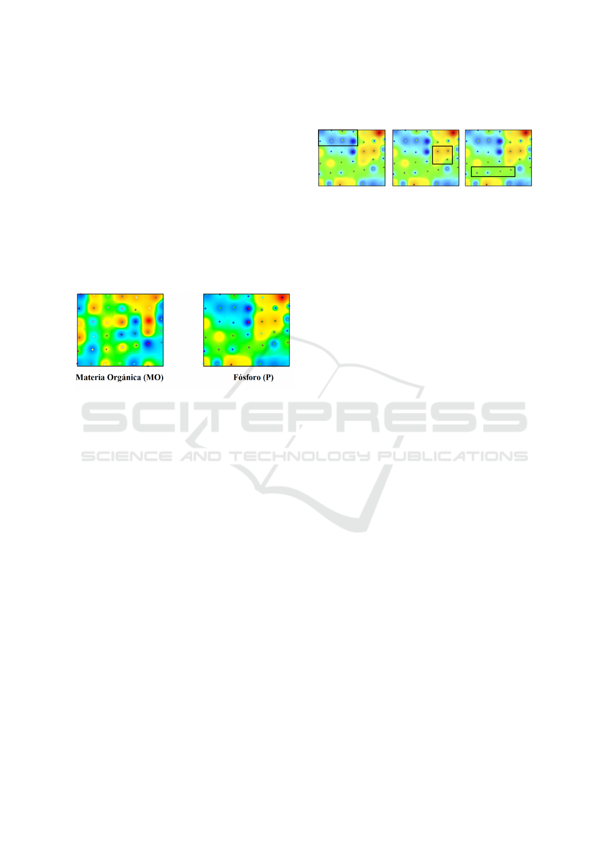
rus, base sum, crop yield, etc. As an example, Figure
1 shows two thematic maps from the same field, one
with organic matter (MO) and the other with phos-
phorus (P). In MO case, green zones represent nor-
mal levels of MO, while red and yellow zones repre-
sent zones with 34.8% and 3.97% above normal val-
ues of MO, also sky blue and blue zones presents val-
ues with 6.06% and 30.68% under normal MO values.
On the other hand, in P case red and yellow zones
are 279.31% y 10.34% above normal, and sky blue
and blue zones are 13.79% y 48.27%, respectively.
Both maps show spatial variability of these indices in
a field, this proves the importance of dividing the field
into management zones with uniform characteristics,
to apply inputs needed in each zone through site spe-
cific farming.
Figure 1: Organic matter and phosphorus map.
Also, we need to include variability in time of the
measured indices. For that, we use thematic map data
sets from the same field for several time periods; these
will be used either to generate the probability distribu-
tion function of the soil property or to create different
scenarios with each one of these instances. A possible
value of the random variable consist in assign a spe-
cific value to each of the sample points on the field,
i.e., the random variable is represented by a vector
that includes each one of the sample points; this vec-
tor has a finite number of possible values. Scenario
probabilities are assigned depending on the number
of instances and the time between each sampling pro-
cess. It is important to notice that a field partition is
a medium term decision, i.e. this partition will last
a specific number of years and after that horizon is
reached, another partition must be set, thus the model
must take into account possible changes in soil prop-
erties during this time. This article uses only histor-
ical data for scenario creation, but it is also valid to
consider forecasts for future periods in the scenario
creation step, but this exceeds the purpose of this ar-
ticle.
Finally, potential management zones are gener-
ated (Z set) through an algorithm that uses all sample
points (S set) as inputs. As an example, in Figure 2
there is an instance with 42 sample point field (6 rows
and 7 columns) and three potential management zones
from a total of 588, each one of them has rectangular
form and includes at least one sample point.
Figure 2: Potential management zones example.
A relationship matrix C = (c
sz
) is created from po-
tential zones generation, where c
sz
= 1 means that po-
tential zone z includes sample point s, and c
sz
= 0 oth-
erwise, for every z ∈ Z, s ∈ S. Besides, index variance
σ
zω
2
is obtained for each potential quarter z and each
scenario ω ∈ Ω, where Ω is the set of possible scenar-
ios. Both parameters are used in the model presented
in the following section.
2.2 Optimization Model
Proposed model consist in a two stage integer
stochastic linear programming model with recource.
In the first stage, the problem minimizes the number
of management zones or quarters that cover the entire
field. In the second stage, the problem minimizes
noncompliance of the homogeneity level using
looseness variables for each scenario but with a
penalty cost for using them. This second stage is
necessary because field partition must be chosen
before knowing random variables performance, and
it must satisfy the homogeneity constraint for any
scenario, this is achieved by minimizing the expected
value of the penalty for the noncompliance of the
homogeneity level.
Sets, parameters and variables used in the model
are described below:
Sets:
Z: set of potential quarters, with z ∈ Z.
S: set of sample points of the field, with s ∈ S.
Ω: set of possible scenarios, with σ ∈ Ω.
Parameters:
c
sz
: Coefficient that represents if quarter z covers
sample point s or not.
M: Penalty cost per unit for noncompliance of the
required homogeneity level.
n
z
: Number of sample points in quarter or manage-
ment zone z.
p
w
: Probability of scenario ω.
σ
2
zω
: Quarter variance z calculated from the soil
property in scenario ω.
σ
2
T ω
: Total variance of the field calculated from the
soil property data in scenario ω.
Delineation of Rectangular Management Zones Under Uncertainty Conditions
273

N: Total number of sample points.
UB: Upper bound for the number of quarters chosen.
α: Required homogeneity level.
Decision variables:
q
z
=
1, if quarter z is assigned to field partition
0, otherwise
h
ω
: Looseness for the homogeneity level in
scenario ω.
The two stage stochastic model with recource is
presented now:
Min
∑
z∈Z
q
z
+
∑
ω∈Ω
p
ω
Q(q, h
ω
) (1)
s.t.
∑
z∈Z
c
sz
q
z
= 1 ∀s ∈ S (2)
∑
z∈Z
q
z
6 U B (3)
q
z
∈ 0, 1 ∀z ∈ Z (4)
W here Q(q, h
ω
) = MinM
ω
h
ω
(5)
s.t.
h
ω
>
∑
z∈Z
[(n
z
− k)σ
2
zω
(6)
+(1 − α)σ
2
T ω
]q
z
− (1 − α)σ
2
T ω
N
h
ω
> 0 (7)
Problem (1)-(4) correspond to the first stage de-
cision, while (5)-(7) correspond to the second stage
decision. Objective function (1) minimizes the sum
of quarters chosen and minimizes the expected value
of the penalty cost for noncompliance of the required
homogeneity level, these are first and second stage
objective functions respectively. Constraint (2) is typ-
ical for set partition models, guarantee that each sam-
ple point on the field is assigned only to one quar-
ter. Constraint (3) establishes an upper bound to the
number of quarters chosen to divide the field. Con-
straint (4) defines that quarter variables must be bi-
nary. Objective function (5) represents second stage
decision for each scenario. Constraint (6) states that
a required homogeneity level must be accomplished;
this constraint is made from the linear version of the
relative variance concept and a looseness variable for
each scenario. Finally, constraint (7) states nature of
second stage variables.
It is important to notice that this model, as in (Al-
bornoz et al., 2013), uses an equivalent linear version
of the constraint related to the relative variance con-
cept. However in this case, as we have different pos-
sible scenarios, we must meet homogeneity level in
each one of these scenarios, thus we will have a rela-
tive variance constraint for each scenario. As we have
to choose only one field partition we need a way to
deal with uncertainty because otherwise we will have
to choose the best field partition for worst possible
scenario in terms of relative variance. We propose
to add new variables named as looseness variables as
part of the second stage decision to get a solution that
considers all possible scenarios, meeting the required
homogeneity level in each one of these, and without
being forced to solve the problem for the worst sce-
nario.
Constraint (6) is created from the following non-
linear constraint used in (Albornoz et al., 2013) :
1 −
∑
z∈Z
(n
z
− k)σ
2
z
q
z
σ
2
T
[N −
∑
z∈Z
q
z
]
> α (8)
This constraint uses relative variance concept, pre-
sented in (Ortega and Santibanez, 2007), is a widely
used criteria to measure effectiveness of chosen man-
agement zones and it must be equal or higher to a
given value, which is the required homogeneity level,
that should be at least 0.5 to validate an ANOVA test
hypothesis assuming k degrees of freedom. To create
constraint (6) first we need to linearize equation (8)
obtaining the following expression:
(1 − α)σ
2
T
[N −
∑
z∈Z
q
z
] >
∑
z∈Z
(n
z
− k)σ
2
z
q
z
(9)
Then if we reorder equation (9) we obtain:
∑
z∈Z
[(n
z
− k)σ
2
z
+ (1 − α)σ
2
T
]q
z
6 (1 − α)σ
2
T
N (10)
As we have a number of possible scenarios we
define a relative variance constraint for each one of
these, and also different parameters for each scenario
ω:
∑
z∈Z
[(n
z
− k)σ
2
zω
+ (1 − α)σ
2
T ω
]q
z
6 (1 − α)σ
2
T ω
N (11)
Here is when we add the looseness variables h
ω
to
the right side of equation (11):
∑
z∈Z
[(n
z
− k)σ
2
zω
+ (1 − α)σ
2
T ω
]q
z
6 (1 − α)σ
2
T ω
N + h
ω
(12)
These variables allow the problem to choose a
field partition that considers all possible scenarios and
meet all relative variance constraints by relaxing the
right side of equation (11) for each scenario, thus fi-
nally obtaining constraint (6). It is important to notice
that looseness variables are added to the linear version
of this constraint to have only linear constraints in the
model.
ICORES 2016 - 5th International Conference on Operations Research and Enterprise Systems
274
3 RESULTS
To analyze the model behavior we used 10 instances
for the problem, each one of them with a different
number of sample points and using crop yield as soil
property because this index has strong variability
in time. In each instance, there are six possible
scenarios, all of them with similar probabilities,
where the two latest scenarios have are more likely to
occur. Chosen parameter values for problem (1)-(7)
are:
M
ω
= 1.5 ∀ω ∈ Ω UB = 40
α = 0.9
p
ω
= 0.15 ω ∈ 1..4
p
ω
= 0.2 ω ∈ 5..6
The rest of the parameters are calculated
from crop yield data for each scenario. The number
of potential quarters is obtained by the formula
((n+1)n(m+1)m)
4
presented in (Albornoz and Nanco,
2015), where n is the number of sample points in
length and m is the number of sample points in width.
Instances used have a different number of potential
quarters, starting from 588 to 13915.
3.1 Instance Solving
Instances were solved with the parameter values de-
fined in this section and using compact equivalent de-
terministic reformulation of the model (1)-(7) using
Cplex 12.4 as a solver in a Lenovo with Intel core i3-
2310M processor CPU 2.10 GHz and a 4 GB RAM
memory. Results are showed in Table 1.
First column indicates the instance number. Sec-
ond column shows total number of sample points on
the field. Third column indicates the number of po-
tential quarters. Fourth column shows stochastic so-
lution of the model. Fifth column is related to the ex-
pected value of perfect information (EVPI), which is
the maximum willingness to pay for knowing all the
information related to random variables performance.
More precisely, this can be calculated using the fol-
lowing formula:
EV PI = RP − W S
Where RP is the optimum value of model (1)-(7)
and WS is the wait-and-see solution, which consid-
ers solving the model for each scenario separately and
then compute the expected value of this solution. At
last, sixth column shows the percentage that EVPI
represents from objective value function. It is im-
portant to notice that EVPI represents between 50%
and 60% of objective value function, this means that
willingness to pay for knowing random variables per-
formance is really high, all of this due to the differ-
ence between scenario solutions and stochastic solu-
tion. This is because stochastic solution must face
any possible scenario so it needs more quarters than
the individual solutions.
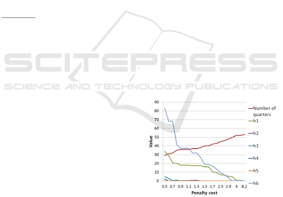
3.2 Sensitivity Analysis of Penalty Cost
Penalty cost is the coefficient related to the loose-
ness variables in the objective function in the second
stage of the problem, thus if this cost is high or low,
looseness variables will have a lower o higher value,
and more or less quarters will be chosen respectively.
For sensitivity analysis we chose instance 9, using the
same parameters as we defined at the beginning of
section 3. In this analysis we use the same value for
every penalty cost M
ω
in each scenario. Table 2 sum-
marizes results achieved.
First column of Table 2 indicates the defined
value of penalty cost. Second column shows total
number of quarters chosen for the optimal solution
(quarters are related to the first stage decision). From
third to eighth column looseness variables from the
second stage for each scenario are showed. Finally
ninth column indicates the stochastic solution of the
model (1)-(7).
Figure 3 shows behavior of the number of quar-
ters chosen while penalty cost changes, it also shows
looseness variables behavior.
It is important to notice when penalty cost raises,
Figure 3: Solution behavior for different penalty costs M
ω
.
looseness variables value decrease and at the same
time the number of quarters increases to satisfy homo-
geneity level constraints. Looseness variables value
decreases at a higher rate than number of quarters in-
crease, this is because when penalty cost is getting
higher it increases the impact of looseness variables
in the objective function. There is a breaking point
Delineation of Rectangular Management Zones Under Uncertainty Conditions
275

Table 1: Instance solution results.
Instance Sample Points Potential Quarters RP EVPI Percentage of O.F.
1 42 588 17.483 8.663 49.6 %
2 80 1980 29.952 15.991 53.4 %
3 100 3025 37.989 21.656 57.0 %
4 120 4290 45.531 27.307 60 %
5 140 5775 49.946 30.327 60.7 %
6 150 6600 52.586 33.125 63 %
7 160 7480 51.458 32.377 62.9 %
8 180 9405 50.817 31.974 62.9 %
9 200 11550 47.931 30.235 63.1 %
10 220 13915 43.999 27.49 62.5 %
Table 2: Sensitivity analysis for the penalty cost M
ω
.
M
ω
Number of quarters h
1
h
2
h
3
h
4
h
5
h
6
F.O.
0.5 29 34.050 2.172 4.951 0 0 83.679 38.363
0.6 31 28.834 0 2.832 0 0 68.119 39.980
0.7 32 20.531 0 0.627 0 0 68.374 41.400
0.8 35 20.292 0.033 1.150 0 0 41.425 42.548
0.9 36 17.924 0.321 0 0 0 37.280 43.496
1 36 17.924 0.321 0 0 0 37.280 44.329
1.1 36 17.924 0.321 0 0 0 37.280 45.162
1.2 37 17.244 0.704 0 0 0 31.714 45.939
1.3 37 17.244 0.704 0 0 0 31.714 46.684
1.4 38 17.430 0 0 0 0 27.182 47.368
1.5 40 16.245 0 0 0 0 19.005 47.931
1.6 40 16.245 0 0 0 0 19.005 48.460
1.7 42 10.198 0 0 0 0 16.861 48.900
2 43 9.590 0 0 0 0 13.567 49.947
2.3 45 7.1226 0 0 0 0 9.468 50.724
2.6 46 6.656 0 0 0 0 7.237 51.418
2.9 48 5.299 0 0 0 0 3.726 51.926
3 50 4.514 0 0 0 0 0 52.031
4 52 0.792 0 0 0 0 0.289 52.649
8 52 0.792 0 0 0 0 0.289 53.297
8.2 53 0 0 0 0 0 0 53
where penalty cost is 8.2, from this point it is not fea-
sible to use looseness variables in problem solution
because is more expensive than use more quarters,
when this occurs then the problem chooses a field
partition based only on the worst scenario in terms
of space variability, this way, required homogeneity
level is reached in every scenario in exchange of a
field partition with a higher number of quarters com-
pared to the other cases with lower penalty cost.
4 FUTURE WORKS
This article covers small and medium size instance
solving by the complete enumeration of all potential
quarters, this also needs computation of parameters
described in section 2.1 for each potential quarter.
This is not feasible for large instances due to the prob-
lem is np-hard and the number of variables increases
really fast when the problem gets bigger, thus we need
more computational effort to calculate all the param-
eters for each variable.
To deal with this issue, we propose to design a de-
composition method based in column generation to
solve large instances without using all the problem
variables. This will be developed based on the de-
composition of the deterministic version of the model
presented in this article, see (Albornoz and Nanco,
2015), because structure is similar, and quarters can
be added as columns in the algorithm as well. This
work is currently being done and it will be included
in a new article.
ICORES 2016 - 5th International Conference on Operations Research and Enterprise Systems
276

5 CONCLUSIONS
This work presents a two stage stochastic linear
programming model with recource to approach the
field partitioning problem facing uncertainty condi-
tions represented by a soil property, which presents
variability in time and is modeled by a set of possible
scenarios. Proposed model solution defines an
optimal field partition that considers every possible
soil property value and as a recource it considers
looseness variables that help to achieve the required
homogeneity level. The model was applied to ten
different instances, and it showed that stochastic
solution is completely different from individual
scenario solutions; this is validated by the EVPI value
in each instance, concluding that a stochastic model
is a better choice than a deterministic one. Besides,
from sensitivity analysis we can conclude when
penalty cost raises, looseness variables use decrease
at a faster rate than the number of quarters increase.
Studied instances in this article were solved by the
complete enumeration of all the potential quarters,
but this is only feasible for small and medium size
instances because the number of potential quarters
grows exponentially as the number of sample points
increases. For this, problem size increases faster than
the sample points increase on the field and a column
generation algorithm will be required to solve large
instances. Also there is another complex situation
when a greater number of scenarios are modeling the
random variables, these aspects will be considered in
future works.
ACKNOWLEDGEMENTS
This research was partially supported by Direccion
General de Investigacion y Postgrado (DGIP) from
Universidad Tecnica Federico Santa Maria, Grant
USM 28.15.20. Jose Luis Saez wishes to acknowl-
edge the Graduate Scholarship also from DGIP.
REFERENCES
Ahumada O., Villalobos J. R., Mason A. N. (2012), Tactical
planning of the production and distribution of fresh
agricultural products under uncertainty. Agricultural
Systems 112, 1726.
Albornoz V. M., Cid-Garcia N. M., Ortega R., Rios-Solis,
Y. A. (2013). Rectangular shape management zone de-
lineation using integer linear programming. Comput-
ers and Electronics in Agriculture 93, 1-9.
Albornoz, V.M., Cid-Garcia, N.M., Ortega, R. and Rios-
Solis, Y.A. (2015). A hierarchical planning scheme
based on precision agriculture. In Handbook of Oper-
ational Research in Agriculture and the Agri-Food In-
dustry, Pla-Aragones, L.M. (Ed.), 129-162, Springer.
Albornoz, V.M. and Nanco, L.J. (2015) An empirical design
of a column generation algorithm applied to a man-
agement zone delineation problem. Lecture Notes in
Economics and Mathematicasl Systems, to appear.
Birge, J. and Loveaux, F. (2011). Introduction to Stochastic
Programming. 2nd ed., New York: Springer.
Bravo M., Gonzalez I. (2009). Applying stochastic goal pro-
gramming: A case study on water use planning. Euro-
pean Journal of Operational Research 196, 11231129.
Gassmann, H.I and Ziemba, W.T. (2012). Stochastic Pro-
gramming. Applications in Finance, Energy, Planning
and Logistics. World Scientific Publishing Company.
Haghverdi A., Leib B.G., Washington-Allen R.A., Ayers
P.D., and Buschermohle M.J. (2015) Perspectives on
delineating management zones for variable rate irriga-
tion. Computers and Electronics in Agriculture 117,
154-167.
Higle, J.L. (2005). Stochastic Programming: Optimization
when uncertainty matters. Tutorials in Operations Re-
search. INFORMS, New Orleans.
Itoh T., Ishii H., Nanseki T. (2003), A model of crop plan-
ning under uncertainty in agricultural management.
Int. J. Production Economics 8182, 555558.
Jaynes D., Colvin T., Kaspar T., (2005). Identifying poten-
tial soybean management zones from multi-year yield
data. Computers and electronics in agriculture 46 (1),
309327.
Jiang Q., Fu Q., Wang Z. (2011). Study on delineation
of irrigation management zones based on manage-
ment zone analyst software. Computer and Comput-
ing Technologies in Agriculture IV, 419427.
Li M., Guo P., (2015), A coupled random fuzzy two-stage
programming model for crop area optimizationA case
study of the middle Heihe River basin, China. Agri-
cultural Water Management 155, 5366.
Liu J., Li Y.P., Huang G.H., Zeng X.T., (2014). A dual-
interval fixed-mix stochastic programming method for
water resources management under uncertainty. Re-
sources, Conservation and Recycling 88, 5066.
Ortega J.A., Foster W. and Ortega R. (2002). Definition
of sub-stands for Precision Forestry: an application
of the fuzzy k-means method.Ciencia e Investigacin
Agraria 29 (1), 3544.
Ortega. R. & Santibanez, O. A. (2007). Determination of
management zones in corn (Zea mays L.) based on
soil fertility. Computers and Electronics in Agricul-
ture, 58, 49-59.
Ramos, A., Alonso-Ayuso, A. and Perez, G.(2008). Op-
timizacion bajo incertidumbre. Espaa, Biblioteca
Delineation of Rectangular Management Zones Under Uncertainty Conditions
277

Comillas. Publicaciones de la Universidad Pontificia
Comillas.
Ruszczynski A. and Shapiro A.(2003). Stochastic Program-
ming. Handbooks in Operations Research and Man-
agement Science, Vol. 10. New York, North-Holland.
Wallace S.W. and Ziemba W.T. (2005). Applications of
Stochastic Programming. MOS-SIAM Series on Op-
timization.
Wiedenmann S., Geldermann J. (2015). Supply planning
for processors of agricultural raw materials. European
Journal of Operational Research 242, 606619
Zeng X., Kang S., Li F., Zhang L., Guo P. (2010). Fuzzy
multi-objective linear programming applying to crop
area planning. Agricultural Water Management 98 ,
134142.
ICORES 2016 - 5th International Conference on Operations Research and Enterprise Systems
278
