Police Officer Dynamic Positioning for Incident

Response and Community Presence

Using Maximum Demand Coverage and Kernel Density Estimation to Plan Patrols

Johanna Leigh, Lisa Jackson and Sarah Dunnett

Department of Aeronautical and Automotive Engineering, Loughoborugh University, Loughborough, U.K.

Keywords: Maximum Coverage Location Problem, Hotspots, Kernel Density Estimation, Tabu Search.

Abstract: Police Forces are under a constant struggle to provide the best service possible with limited and decreasing

resources. One area where service cannot be compromised is incident response. Resources which are

assigned to incident response must provide attendance to the scene of an incident in a timely manner to

protect the public. To ensure the possible demand is met maximum coverage location planning can be used

so response officers are located in the most effective position for incident response. This is not the only

concern of response officer positioning. Location planning must also consider targeting high crime areas,

hotspots, as an officer presence in these areas can reduce crime levels and hence reduce future demand on

the response officers. In this work hotspots are found using quadratic kernel density estimation with

historical crime data. These are then used to produce optimal dynamic patrol routes for response officers to

follow. Dynamic patrol routes result in reduced response times and reduced crime levels in hotspot areas

resulting in a lower demand on response officers.

1 INTRODUCTION

Police forces must operate to a high efficiency to

ensure the safety of the public and property with the

limited budget available. In many countries the

police are currently facing budget cuts and hence

this is of increasing importance. One area where the

public’s safety is very reliant on efficient use of

resources is incident response. This is where a

situation is brought to the attention of the police

dispatchers and it is determined that an officer

presence is required at the situation. An officer out

of those assigned to response is then allocated to the

situation. An example of this could be when a

burglary is reported to be currently taking place. In

this situation resources will be allocated to attend the

incident with the aim of apprehending the criminal.

The time taken to reach the scene of the incident can

affect the outcome of the situation. In the UK there

are target response times which are dependent on the

incident severity and whether it occurs in the city or

rural environment. To increase the chances of an

officer being able to respond to an incident within

these response times their positioning whilst not

attending an incident can be optimized. The key

factors to consider when positioning officers are:

 predicted demand coverage

 presence in areas where crime levels are

high

 visibility.

The first key factor requires the officers, not

currently attending an incident, to be positioned to

give the highest possible demand coverage. Hence

this aspect of positioning is considered as a

maximum coverage location problem, using an

advancement of the double standard model used

previously for ambulance positioning (Gendreau et

al., 1997). The method varies from the original to

allow the response time restrictions for both city and

rural areas to be considered. Though demand

coverage is a major concern it is not the only

concern when positioning police officers. It has been

shown that a police presence in areas of high crime,

hotspots, can reduce crime in that area (Smallwood,

2015). The visible presence of a police officer also

increases the public’s feeling of safety. Due to the

need to visit hotspots and visibility requirements

police officers cannot be positioned by only

considering the ideal response location. Hence in

this work a method of dynamic patrol route planning

is developed, that takes into account demand

Leigh, J., Jackson, L. and Dunnett, S.

Police Ofﬁcer Dynamic Positioning for Incident Response and Community Presence - Using Maximum Demand Coverage and Kernel Density Estimation to Plan Patrols.

DOI: 10.5220/0005705402610270

In Proceedings of 5th the International Conference on Operations Research and Enterprise Systems (ICORES 2016), pages 261-270

ISBN: 978-989-758-171-7

261

coverage, hotspots and visibility to determine the

most efficient route for officers to take when

patrolling. This model of patrol planning also

considers those response officers not presently

available to patrol by removing them from the

directed patrol routes whilst still considering them

with regards to demand coverage.

The current method of directing patrol routes in

the UK is through informing officers of waymarker

locations, which are areas of concern, during a

briefing before a shift. They are asked to visit these

and stay within the defined waymarker boundaries

for a set period of time, i.e. 15 minutes, when

possible. They are not advised when to do this,

where other officers are and hence are not

considering demand coverage. This research

demonstrates a method of advising officers on where

to travel in real time when not attending an incident.

This research address an issue experienced by

many police forces and has benefited from

collaboration with Leicestershire police in the UK.

Due to this collaboration Leicestershire has been

used as a case study. Processes may vary slightly

between forces but the tool will still be applicable.

The remainder of this paper is broken up as

follows. Section 2 gives background to the project

through looking at relevant research. Section 3

defines the problem to be addressed and aspects to

consider. Section 4 describes the maximum coverage

location problem to be solved. Section 5 shows how

crime analysis is performed using quadratic kernel

density estimation and how the crime data is

displayed using thematic mapping. Section 6 details

how the location problem is solved using a tabu

search heuristic. Section 7 describes the routing

process between hotspots. Section 8 contains the

results of solving the problem and finally section 9

concludes the paper.

2 LITERATURE REVIEW

Location planning has already been heavily

researched in many areas including ambulance

positioning. These applications are generally looking

at stationary locations. A maximal covering location

problem (MCLP) is used to find the optimal location

for ambulances (Daskin and Stern, 1981). This study

is relevant to the police demand coverage problem

but does not consider the two time restrictions

required in police coverage and does not consider

that repositioning is required. The MCLP problem is

advanced to consider two time standards and the

different levels of demand coverage required in the

double standard model (Gendreau et al., 1997). This

does not consider the two time restrictions required

by the police. Further studies also considers the

MCLP but considers repositioning when an

ambulance is sent to an incident (Mandell, 1998).

The study also considers the availability of the

servers and two different servers. This study is

relevant when considering the conditions of moving

officers but does not consider the different level of

coverage required and that police should not revisit

bases within a certain time.

Operation Savvy (Smallwood, 2015) is a police

operation carried out by West Midlands Police and

Cambridge University to investigate the effect of

directed patrols on crime hotspots. These directed

patrols consisted of police community support

officers (PCSOs) visiting the epicentre of a hotspot

for fifteen minutes, three times at prime time, which

is between 3pm and 10pm Wednesday to Saturday.

To form the hotspots demand data from two years

was used in a 150m radius. The hotspots focused on

in this study are anti-sociable behaviour (ASB),

burglary, criminal damage, theft and vehicle crime.

Patrols were stepped up in 40 hotspots and 40

hotspots were kept as controls. The results of this

study showed that in the high and medium crime

level experimental hotspots there was a noticeable

reduction in all crime types and anti-social

behaviour. Further results on the communities trust

and confidence in the police is to be examined by a

survey. This study proved the effectiveness of

directed patrol routes but only used this to direct

PCSO patrols at certain times of day and demand

coverage was not considered.

A tool, GAPatrol, to help police managers plan

patrol routes is proposed in (Reis et al., 2006). In

this study multiagent-based simulation assists in the

design of police patrol routes. The simulation finds

crime hotspots and plans routes with better coverage

in these hotspot areas. Hence the routes are planned

with the single aim of reducing crime levels and do

not consider demand coverage for incident response.

The patrol routes of state troopers concerned

with the prevention of traffic incidents has been

explored (Li and Keskin, 2013). The aim of the

study is to determine the best locations for

temporary stations and increase the effectiveness of

patrols by increasing visibility in time periods where

high levels of crime have been experienced whilst

minimizing associated costs which include price of

state troopers, travelling costs and station fees. The

problem to be solved is similar to a multi-depot,

dynamic location and routing problem.

A previous study on planning patrol routes based

ICORES 2016 - 5th International Conference on Operations Research and Enterprise Systems

262

patrol routes on giving each road a crime rating and

visiting those with the highest costs whilst also

keeping cost of travel low (Chawathe, 2007). This

study does not consider demand coverage for

incident response and also only considers one police

unit at a time which is not practical. In reality there

are many units and where each of these units are

patrolling effects the other units.

An alternative study on patrol routes uses ant

colony algorithms along with Bayesian decision tool

to plan patrol routes (Chen et al., 2015). The ant

colony aspect relates to the history of patrols being

tracked by the drop of virtual pheromone and its

decay. This is a good method of stopping repeat

hotspot visiting within short spaces of time whilst

also tracking when another visit is required. The

downfall of this study is that it doesn’t consider

coverage for incident response.

These previous studies help develop the idea of a

dynamic routing problem addressed in this research.

Once the problem is formulated a method of Tabu

search is considered to solve the problem using

MATLAB. Tabu search allows the search area to be

narrowed down to give a solution in a shorter

computational time, which is required in the fast

paced dispatch process.

Hotspot mapping is a means of analyzing historic

crime data to predict future crime patterns. This is

possible as crime is not random. Crime follows

patterns due to environmental influences effecting

criminal’s decisions (Kennedy et al., 2011). Crime

mapping is widely used within the police and law

enforcement agencies. There are many different

methods including point mapping, spatial ellipses,

thematic mapping and Kernel Density Estimation.

There have been many studies determining the best

method of hotspot mapping. A study by (Chainey et

al., 2008) identified Kernel Density Estimation as

the best method for predicting future crime

locations. Hence it is the method which will be used

in this study.

3 PROBLEM FORMULATION

A response officer’s main duty is to provide

emergency response to incidents of high severity.

Responding to incidents takes up the majority of

their time and there is limited time to patrol. When

there is time to patrol these patrols must be directed

efficiently. Those officers whom require patrol

direction are those which are not currently attending

an incident. The problem investigated is improving

the efficiency of these patrol routes by giving them

direction in real time. This direction is based on

keeping good demand coverage between all the

response officers and being visible in problem areas,

hotspots. This will keep response times low and in

the process deter crime from hotspots.

Response officers operate in units as some are

paired to create double crewed vehicles hence the

entities considered are response units. When a

response unit is free to patrol the location to patrol is

calculated using the processed formed in this

research. The chosen location is then conveyed to

the response unit as simple instructions. These

instructions include time to spend at the location and

what to look for, it assumed the unit will take the

quickest route to this incident hence directions are

not necessary. When they have attended the hotspot

for the appropriate length of time this hotspot is

marked as visited and if required a new hotspot

location is assigned to the response unit. As more

response units become free they are allocated

hotspots. If incidents arise within the patrolling time

the response to incident will take priority.

When solving the problem there are some

constraints to be considered regarding policing

standards and processes. Leicestershire Police

requires that in an emergency situation a unit should

attend the incident within fifteen minutes, which is

taken to be 



, in heavily populated areas such as

cities and towns. In sparsely populated areas such as

rural areas the response time should be within

twenty minutes, which is taken to be 



. The area

can then be divided into areas with a node at the

centre. Hence a node is considered covered if the

following conditions are met:

 when considering a town/ city a unit must be

located within 



of node 

 when considering a rural area a unit must be

located within 



of node

Taking the distance which can be travelled within





to be 



and within 



to be 



where 









(Mandell, 1998).

This is a spatial problem which requires a region

to be used for modelling. Data from

OpenStreetMaps (© OpenStreetMap contributors,

2015) is used to form a directed graph of the roads in

Leicestershire within MATLAB. The road map

formed is shown in figure 1.

The problem formulated is now considered as a

MCLP using hotspots as possible nodes to locate

response units.

Police Ofﬁcer Dynamic Positioning for Incident Response and Community Presence - Using Maximum Demand Coverage and Kernel

Density Estimation to Plan Patrols

263

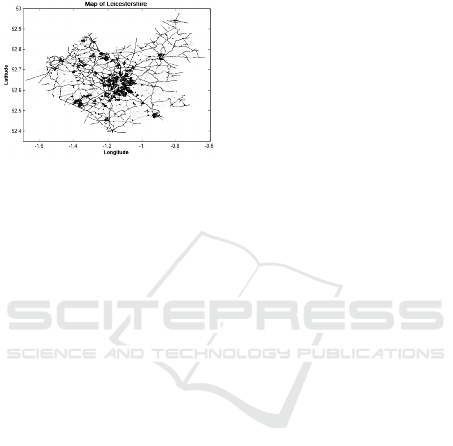
Figure 1: Road map of Leicestershire.

4 MAXIMUM COVERAGE

LOCATION PROBLEM

Demand coverage is a measure of how well response

units are able to cope with possible emergency

response demand. This can be determined by

predicting demand using historical incident data and

whether an officer can reach the demand location,

node , within the recommended response time.

Nodes are a point of reference to measure demand

from, they can be a point on a street or in reference

to an area.

A variation of the double standard model is used

to find maximum police coverage for a given

number of officers (Gendreau et al., 1997). This

method is suitable as it considers two time standards

and also allows different levels of coverage, , to be

considered. This is necessary because areas with

high levels of demand are not sufficiently covered

by one response unit.  allows the level of response

units required to consider a region as covered to be

set. The objective function for this is equation (1)

which aims to maximize coverage. The demand

points are represented by the set 







,



,…,





and the demand at these points is 



. 





is a binary

variable which equals 1 if 



is covered a minimum

of k times within the radius 



and 0 otherwise.

Where k is the number of units which are in range to

reach node .

Maximize

∑











∈

(1)

This objective function has been adapted here to

apply to the police positioning problem. The

adaption is necessary to account for the

recommended response times for city and rural

areas. Equation (2) accounts for city and rural

response guidelines. In this equation 









is a binary

variable which equals 1 if 



is covered a minimum

of k times within the radius 



. 









is a binary

variable which equals 1 if 



is covered a minimum

of k times within the radius 



. C and R are binary

variables which equal 1 if node 



is in a city or rural

area.

Maximize

∑































∈

(2)

The objective function results in the total demand

covered at least k times within the required

emergency response distances, 



or 



depending on

its location. It is subject to the constraints:





1 



∈



∈





(3)







,







,









∈



(4)





∈



(5)









,





∈



0,1













∈



(6)

,∈



0,1



(7)

1

(8)

When considering response unit positioning 







,



,…,





represents the set of possible

locations, these are decided by the hotspots found

from incident analysis. 



shows the number of

resources located at . The total number of units

available is taken to be  and this is determined by

the number of officers on shift with an available

status at that time, whether they are single or double

crewed and their availability. These constraints also

differ from the original double standard model due

to the different priorities of the police (Gendreau et

al., 1997). The problem will still aim to cover all

demand within at least 



which is taken into account

by constraint (3). Constraint (4) states that node

can only be covered +1 times if it is covered at

least  times. Constraint (5) ensures that the sum of

all the officers at each point W is equal to .

Constraint (6) and (7) ensures 









,









,  and  are

binary values. Finally constraint (8) states that either

 or  must equal 1, but never both at the same

time.

When solving the objective function above there

are rules on where each officer can be placed due to

their status and attached station. These are:

1. An officer can only move if its status is available

(they are not attending an incident, in custody, on

a break, etc.).

2. An officer only counts as covering an area if they

are free to attend an incident, this includes

officers who are available or attending an incident

ICORES 2016 - 5th International Conference on Operations Research and Enterprise Systems

264

more minor than an emergency incident.

3. The distance from their base police station must

be less than maximum displacement from their

station allowed 







, where 



is the distance

from the base police station to the possible

location where an officer is required and 



is the

maximum distance an officer is allowed from

their base station determined by the police force.

Rule 1 is just the condition that a police officer must

be available before moving them. In rule 2 an officer

is counted as covering an area if attending a grade 2

incident because if necessary they can leave such an

incident to respond to an emergency incident but

they cannot be moved unnecessarily. Hence they are

not moved when solving for maximum coverage.

Rule 3 ensures that officers do not move too far

from their base police station. Each officer has an

attachment to a particular police station and even

though most police forces operate as boundaryless

within their area it is not efficient to move an officer

too far away from their associated station due to

their journey back at the end of a shift.

When applying this approach to the ambulance

location problem the possible nodes () where they

can be located are bases, such as car parks and

service stations. For the police it is more important

to be based in hotspot areas where they are a

deterrent to further crime.

5 INCIDENT MAPPING

Location is a very important factor when analyzing

crime as repeat area targeting is more common than

repeat offenders. Crime mapping is used to show

where crimes occur; this allows the movement of

crime over time to be analyzed. A study previously

discussed (Reis et al., 2006) showed that crime is not

evenly distributed but forms patterns due to the

habits of criminals. Figure 2 shows the crime spread

through Loughborough (a small town within

Leicestershire) by the numbers in grey circles. It

demonstrates the uneven distribution of crime, for

example the town centre has a high level of crime at

119 incidents (Police UK, 2015). Crime analysis

identifies these patterns which is the first step in

reducing crime levels. Crime analysis is vital in the

planning of patrol routes as routes should be directed

to visit areas of higher than average levels of crime,

called hotspots.

Finding hotspots, determining the causes and

responding to the results to reduce crime in the areas

identified is referred to as problem oriented policing.

Figure 2: Crime distribution.

Crime analysis has been in police forces for a long

time, beginning with a map with pins in to represent

crimes, developing to the same concept on a

computer. It has been proven that focused patrols

depending on these hotspots can assist with the

prevention of crime (Smallwood, 2015). Currently

police forces have a crime analysis team to look into

crime patterns and computer programs to determine

where high levels of crime occur.

Before crime can be analysed it requires filtering

to pick out the data which is relevant to the problem

and to discard bad data. This is described in section

5.1. Once it has been filter a means of analysing it is

required which is done using quadratic kernel

density estimation in section 5.2.

5.1 Incident Data Analysis

Data analysis is required to filter the

incidents/crimes down to those relevant to police

patrolling. The crimes and incidents considered are

those where the presence of an officer can help deter

them. These include:

 anti-social behavior

 theft

 vehicle crime

 burglary in dwelling and other

 criminal damage.

Incidents in certain places should be excluded

from the analysis as they also cannot be prevented

by the presence of an officer patrolling on the

streets, these places include:

 clubs or bars

 shopping centers

 hospitals.

There are some incidents on record which may

cause anomalies to the hotspot locations this is cases

such as incidents mapping to a default area when the

correct location has not been given. These are also

filtered out before analysis of crime data.

Crime levels change depending on day, time of

Police Ofﬁcer Dynamic Positioning for Incident Response and Community Presence - Using Maximum Demand Coverage and Kernel

Density Estimation to Plan Patrols

265

day and season. Hence it is not accurate to find

general hotspots. Data is separated into Sunday-

Thursday and Friday – Saturday and also into day,

evening and night as well as seasonality. Hotspot

analysis is then carried out separately using only

data from the allocated time period. As hotspots

change with time the possible locations to position

officers (W) vary.

5.2 Kernel Density Estimation

Kernel Density Estimation is a method of spatial

analysis for crime mapping which allows complex

point patterns to be simplified to assist in the

identification of hotspots. This method is superior to

other crime mapping methods as it is not limited by

strict boundaries such as beat boundaries. Beat

boundaries are predefined areas, such as a town,

which an officer has to patrol. Using boundaries can

result in some hotspots which cross the boundary not

being identified. Kernel Density Estimation uses

grids however also considers the areas surrounding

the grid cell, by using kernels, to allow the

surrounding area to influence the intensity of crime

within the cell.

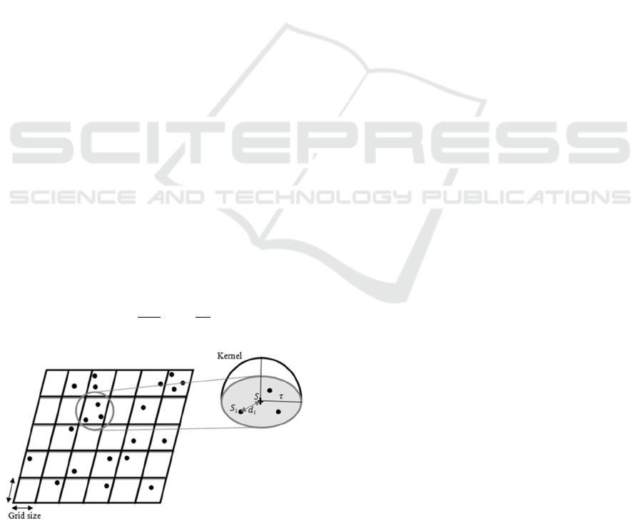
Quadratic kernel density estimation involves

overlaying a grid onto the map and visiting each grid

cell to preform kernel density estimation. Figure 3

shows how quadratic kernel density estimation is

performed and the process is then described below.

Kernel density estimation finds the points at

which crime incidents have occurred within the

predefined bandwidth boundary and determines the

influence each of these crimes has on the intensity of

crime in that area using equation 9 (Gatrell et al.,

1996).



















1





















(9)

Figure 3: Quadratic kernel estimation.

Where 











is the intensity of crimes within the

bandwidth () as a function of the distance from the

center (s). 



is the distance between the grid centre

and the point being investigated.

This intensity is inversely weighted, giving

crimes near the centre of the grid cell a greater

contribution to the intensity than those further from

the centre. As crimes move further from the centre

the intensity decreases until finally those on the

boundary have an intensity of zero.

To perform this successfully an appropriate

bandwidth and grid size must be determined. A

bandwidth too large causes excessive smoothing

which in turn leads to hotspots not being found. A

bandwidth which is too small leads to insufficient

smoothing causing a spikey graph, which leads to

incorrect identification of hotspots. In this work both

the bandwidth and grid cell size are determined

using testing where computational time is taken into

consideration. The resulting bandwidth for this

analysis is taken to be 0.001

and grid cell size

0.001

x 0.001

, measured in the longitude and

latitude coordinate system.

Now the objective function is defined with

constraints and the hotspot locations have been

found the equation can be solved using tabu search.

6 TABU SEARCH

There are many possible solutions to the MCLP. The

ideal situation would be to find the optimal solution

to position officers in the optimal locations. To find

the optimal solution each solution must be

investigated, exhaustive search. Doing an exhaustive

search would take considerable computational time,

making it an impractical approach; hence a method

of narrowing the search is required. Tabu search is a

method of searching for a solution without

investigating every solution. It does not guaranty an

optimal solution but has been proven to be an

accurate method of solving similar problems

(Gendreau et al., 1997). Hence for this problem tabu

search is used to solve the MCLP for police officers.

Tabu search is a form of local search. Local

search has the disadvantage of getting stuck at local

optima, Tabu search stops the search getting stuck at

a local optima as it finds a solution and then moves

from this solution to its best neighbour even if this

causes the objective value to deteriorate which

allows solution to move on from local optima. A

neighbour is a solution one move away from the

previous solution and the best neighbour gives the

maximum value when calculating the objective

functions. Revisiting solutions is stopped by using a

ICORES 2016 - 5th International Conference on Operations Research and Enterprise Systems

266

tabu list, each solution which has been visited is

placed on the tabu list and the solutions on this list

can’t be revisited whilst they remain on the tabu list.

They will remain on the list for a selected number of

iterations.

Response units are advised to remain in the

hotspots they are allocated for a set period of time

determined by the police force, typically 15 minutes.

If a response unit completes the recommended

attendance period of a hotspot this hotspot is marked

as visited. Those hotspots recently completed are

placed on the tabu list to stop response units

revisiting hotspots which have recently been visited

and give preference to choosing those hotspots

which have not recently been visited. This tabu list

is kept through multiple searches. Revisits can be

performed only after a certain period of time which

is dependent on the strength of the hotspot.

6.1 Tabu Search Process

An initial solution is found randomly and solved

using equation (2) and constraints (3)-(8). The

neighbouring solutions are then found which are

found by moving one officer to a new location per

neighbouring solution and they are solved in the

same way. The hotspot locations available to

position officers will be decided depending on the

time of day, day of the week and season. Out of

these the best solution is taken and all others are

added to the tabu list. This stops the solution cycling

back to the same solution and getting stuck at a local

optima. This new solution is taken to be the solution

and the process is restarted. This process is repeated

until one of the stopping criteria is met.

When a stopping criterion is met the best

solution is used to position officers. Once the

appropriate time to visit a hotspot has passed, e.g. 15

minutes, the problem is solved again to re-determine

using the new response unit statuses and locations. A

new tabu list is started prohibiting revisiting hotspots

which have been visited.

6.2 Stopping Criteria

 The maximum number of iterations has been

reached

 The number of iterations since the last

improvement has exceeded a set value

 Optimal solution obtained.

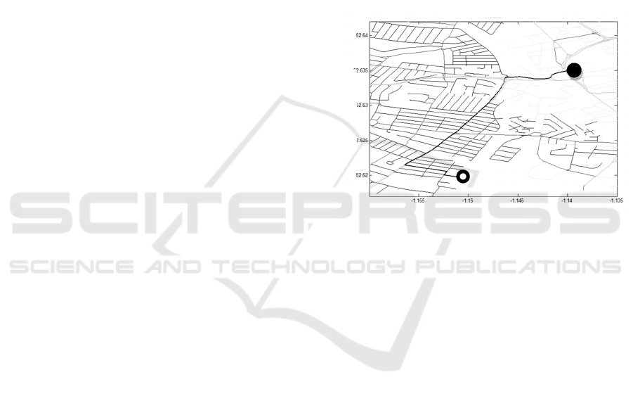
7 ROUTING BETWEEN

HOTSPOTS

The response units are allocated a hotspot to attend

but assumed to take the shortest route to this hotspot.

Which hotspot to allocate to each response unit is

determined by calculating the routes between the

response units and the hotspots which have been

chosen by the MCLP. The solution with the lowest

overall distance travelled whilst meeting all the

constraints is chosen and the response units are

allocated accordingly. The routes are calculated

using Dijkstra’s algorithm.

Figure 4: Patrol route.

Figure 4 represents a typical route between an

officer and a hotspot. The circle with no centre

represents a police officer. The filled circle

represents the centre of the hotspot. The thick black

line details the routes to the hotspots.

8 RESULTS

The resulting process to determine optimal officer

locations is detailed in figure 5. The flow chart

shows that the road map for the region of concern is

developed, the crime data is then filtered and used to

determine hotspots, before being solved as a

maximum coverage location problem. The results

are then conveyed to the response units. The MCLP

is solved each time response units require

positioning. The hotspots are reevaluated regularly,

using the new crime data available, to find new

hotspots.

The officer positioning process is tested by

simulation. The simulation runs through typical

situations which may occur within police response.

The officer positioning tool is used when necessary

Patrol route

Latitude

Longitude

Police Ofﬁcer Dynamic Positioning for Incident Response and Community Presence - Using Maximum Demand Coverage and Kernel

Density Estimation to Plan Patrols

267

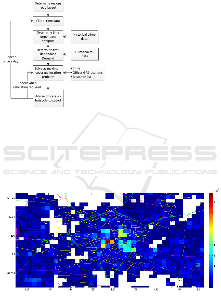
Figure 5: Automated positioning process.

to allocate officers to hotspots. The simulation

demonstrates the ability for the tool to determine

efficient positioning for the officers.

The first section of the processes is identifying

the hotspots. An example of a typical hotspot map

for anti-social behaviour, produced by Kernel

Density Estimation analysis, is shown in figure 6.

The figure shows the hotspots found in Leicester

center during the evenings of Friday and Saturday.

The red square indicates the area with the highest

crime intensity level, followed by orange and

yellow. The shades of blue represent a low crime

intensity level and no colour indicates that there is

no significant case of anti-social behaviour. Out of

all the hotspots identified through kernel density

estimation the top 3% are used as possible locations

to position officers. These hotpots are used to solve

for the objective function. Another grid is overlaid

onto the map which contains the predicted call

demand. This is used to determine what demand is

covered when positioning officers. The number of

officers is taken to be p which is based on the

number of officers on shift and typical availability of

these officers. The population in the area determines

whether the cell is considered rural or city.

The performance of the positioning processes is

currently measured using historical data to prove its

worthiness before testing within police forces. This

is done by running the simulation for a period of

time in history where crime data has been recorded

for. Only crime information recorded before this

period starts can be used in the analysis, to simulate

the fact that when using the positioning tool in real

time the crime data is not available as it hasn’t

happened. The difference is when using a historical

time period the crime data for this period can then be

used to determine how well the officers targeted the

areas which crimes did occur in within this time

period. Hence if the officers had targeted these areas

these are the crimes which the officers may have

prevented. Equation (10) is used to determine how

Figure 6: Thematic map of kernel density results.

Kernel Density Estimation Graph of Leicester Centre

Latitude

Longitude

ICORES 2016 - 5th International Conference on Operations Research and Enterprise Systems

268

accurately the positioning tool targeted crime. The

equation originates from a study by (Chainey et al.,

2008) to determine how efficiently different crime

mapping methods predicted where future crime

occurred. In this case n represents the number of

crimes which occur within the hotspots target by

officers, whilst N is the total number of crimes

which occur. a is the total area of all the hotspots

targeted, whist A is the total area of the region

studied.





100





100

















(10)

Using this equation over a one month period

allowing for 5% of an officers shift time to be

allocated to patrolling resulted in the potential to

deter 22% of street crimes. Increasing the time

available to patrol would increase the ability to deter

crime. Decreasing the time available for officers to

patrol would decrease ability to deter crime.

Tabu search offered a search method with

lower computational costs than performing an

exhaustive search. It did not guarantee the optimal

solution though there wasn’t a significant difference

between the optimal result and the tabu result.

9 CONCLUSIONS

Dynamic directed patrol routes for response officers

are a way of ensuring officers are efficiently placed

for incident response whilst also visiting hotspot

areas. A program which advises officers on where to

patrol is unique and has a place in the current police

objective to work more efficiently using predictive

policing.

The variation of the double standard model

allows both city and rural response time

requirements to be considered. It also allows

different levels for coverage to be accounted for.

Whilst quadratic kernel density estimation

effectively predicts crime hotspots as it reduces

boundary effects by considering the surrounding

areas. This coupled with thematic mapping allows

clear graphical representation of crime hotspots.

Solving quickly is an important aspect of locating

police offices and tabu search gives a shorter

computational time than exhaustive search.

The effects of directing patrol routes include a

decrease in response times and an increased ability

to deter crime. The next stage for this method is to

include more methods of hotspot identification, as

well as testing in real time within a police force

response team. The performance of this method can

then be evaluated by testing within the police force.

Where the performance of hotspot targeting can be

measured by the overall level of crime and the

performance of demand coverage can be measured

by the change in response times.

ACKNOWLEDGEMENTS

The cooperation of the Leicestershire Police is

gratefully acknowledged as without their support

this project would not be possible. This work was

supported by the Economic and Social Research

Council [ES/K002392/1].

REFERENCES

Chainey, S., Tompson, L., Uhlig, S., (2008). The Utility of

Hotspot Mapping for Predicting Spatial Patterns of

Crime. Security Journal, palgrave. Vol. 21, p. 4-28.

Chawathe, S.S. (2007). Organizing Hot-Spot Police Patrol

Routes. Intelligence and Security Informatics, IEEE.

p.79-86.

Chen, H., Cheng, T., Wise, S., (2015) Designing Daily

Patrol Routes for Policing Based on Ant Colony

Algorithm. ISPRS Annals of the Photogrammetry

Spatial Informatics Sciences. Vol. II-4/W2. p. 103-

109.

Daskin, M. S., Stern, E. H., (1981). A Hierarchical

Objective Set Covering Model for Emergency Medical

Service Vehicle deployment. Transport Science,

Institute for Operations Research and the Management

Science. Vol. 15 (Issue 2). p. 137-152.

Gatrell, A. C., Bailey, T. C., Diggle, P. J., Rowlingson,

B.S. (1996). Spatial Point Pattern Analysis and its

Applications in Geographical Epidemiology.

Transactions of the Institute of British Geographers,

Royal Geographical Society. Vol. 21 (Issue 1). p. 256-

274.

Gendreau, M., Laporte, G., Semet, F., (1997). Solving an

Ambulance Location Model by Tabu Search. Location

Science, Elsevier Science Ltd. Vol. 5 (Issue 2). p. 75-

88.

Kennedy, L., Caplan, J., Piza, E., (2011). Risk Clusters,

Hotspots, and Spatial Intelligence Terrain Modeling as

an Algorithm for Police Response Allocation

Strategies. Journal of Quantitative Criminology,

Springer. Vol. 27, issue 3, p. 339-362.

Li, S. R., Keskin, B. B., (2013). Bi-criteria Dynamic

Location-Routing Problem for Patrol Coverage.

Journal of the Operational Research Society,

Operational Research Society. Vol. 65. p. 1711-1725.

Mandell, M., (1998). Covering Models for Two-Tiered

Emergency Medical Services Systems. Location

Police Ofﬁcer Dynamic Positioning for Incident Response and Community Presence - Using Maximum Demand Coverage and Kernel

Density Estimation to Plan Patrols

269

Science, Elsevier Science Ltd. Vol. 6. p. 355-368.

[Online]. Available at: http://

www.openstreetmap.org/#map=10/52.5964/-1.1838.

Police.UK (2015). Loughborough Central. Available at:

http://www.police.uk/leicestershire/L07/

Reis, D., Melo, A., Coelho, A., Furtado, V., (2006).

Towards Optimal Police Patrol Routes with Genetic

Algorithms. Mehrotra, Springer. Vol. 3975. p. 485-

491.

Smallwood, J. (2015) What Works Crime Reduction:

Operation SAVVY [Online]. College of Policing.

Available at: http://whatworks.college.police.uk/

Research-Map/Pages/ResearchProject.aspx?projectid=

306 [Accessed: 08/06/2015].

ICORES 2016 - 5th International Conference on Operations Research and Enterprise Systems

270