
Evolution Strategies and Covariance Matrix Adaptation
Investigating New Shrinkage Techniques
Silja Meyer-Nieberg and Erik Kropat
Department of Computer Science, Universit
¨
at der Bundeswehr M
¨
unchen,
Werner-Heisenberg Weg 37, 85577 Neubiberg, Germany
Keywords:
Evolution Strategies, Covariance Matrix, Adaptation, Shrinkage Estimators.
Abstract:
This paper discusses the covariance matrix adaptation in evolution strategies, a central and essential mecha-
nism for the search process. Basing the estimation of the covariance matrix on small samples w.r.t. the search
space dimension is known to be problematic. However, this situation is common in optimization raising the
question, whether the performance of the evolutionary algorithms could be improved. In statistics, several ap-
proaches have been developed recently to improve the quality of the maximum-likelihood estimate. However,
they are seldom applied in evolutionary computation. Here, we focus on linear shrinkage which requires rela-
tively little additional effort. Several approaches and shrinkage targets are integrated into evolution strategies
and analyzed in a series of experiments.
1 INTRODUCTION
Evolution strategies (ESs) belong to the class of evo-
lutionary algorithms. Their performance compared to
other black-box optimization techniques is good as it
has been observed in practice and in several competi-
tions as e.g. (Hansen et al., 2010). Since they oper-
ate mainly in continuous search spaces, their central
search operator is mutation which is typically real-
ized as a multivariate normal distribution with mean
m and covariance matrix σ
2
C. In order to progress
fast and reliably towards the optimal point, the ex-
tent as well as the directions of the mutations must
be adapted so that the distribution of the random vari-
ables is suitable to fitness landscape of the particu-
lar function. Techniques for controlling the mutation
process have therefore received a lot of attention in
research on evolution strategies. The focus lies on
the control of covariance matrix. The covariance ma-
trix adaptation techniques developed typically make
use of a variant of the sample covariance. However,
the estimation problem is ill-posed: Due to efficiency,
the sample size is relatively small w.r.t. the search
space dimension. This leads to a well-known problem
in statistics: The covariance matrix estimate may dif-
fer considerably from the underlying true covariance
(Stein, 1956; Stein, 1975). Taking a closer look at
the adaptation equations, reveals that nearly all adap-
tation techniques introduce correction or regulariza-
tion techniques by falling back to the previous covari-
ance matrix and/or by strengthening certain promis-
ing directions. These procedures exhibit similarities
to shrinkage estimation in statistical estimation the-
ory leading to the research question of the present pa-
per: If evolution strategies perform a kind of implicit
shrinkage, can they profit from the introduction of ex-
plicit shrinkage operators?
The current analysis extends the work carried out
in (Meyer-Nieberg and Kropat, 2014; Meyer-Nieberg
and Kropat, 2015a) and augments the investigation
conducted in (Meyer-Nieberg and Kropat, 2015b;
Meyer-Nieberg and Kropat, 2015c) for the case of
thresholding estimators. (Meyer-Nieberg and Kropat,
2014; Meyer-Nieberg and Kropat, 2015a) presented
the first approaches to apply Ledoit-Wolf shrinkage
estimators in evolution strategies. There, the shrink-
age estimators were combined with an approach stem-
ming from a maximum entropy covariance selection
principle. A literature review resulted in only two pa-
pers aside from our previous approaches: An applica-
tion in the case of Gaussian estimation of distribution
algorithms albeit with quite a different goal (Dong
and Yao, 2007). There, the learning of the covariance
matrix during the run lead to non positive definite ma-
trices. For this reason, a shrinkage procedure was ap-
plied to “repair” the covariance matrix towards the re-
quired structure. The authors used a similar approach
as in (Ledoit and Wolf, 2004b) but made the shrink-
age intensity adaptable. More recently Kramer con-
sidered Ledoit-Wolf-estimator based on (Ledoit and
Meyer-Nieberg, S. and Kropat, E.
Evolution Strategies and Covariance Matrix Adaptation - Investigating New Shrinkage Techniques.
DOI: 10.5220/0005703201050116
In Proceedings of the 8th International Conference on Agents and Artificial Intelligence (ICAART 2016) - Volume 2, pages 105-116
ISBN: 978-989-758-172-4
Copyright
c
2016 by SCITEPRESS – Science and Technology Publications, Lda. All rights reserved
105

Wolf, 2004a) for an evolution strategy which does not
follow a population-based approach but uses a vari-
ant of the (1+1)-ES with covariance matrix adaptation
for which past search points are taken into account
(Kramer, 2015).
Here, we focus on an approach in the eigenspace
of the covariance matrix. Several shrinkage targets
are analyzed and compared with each other and with
the original ES version. The paper is structured as fol-
lows: First, a brief introduction into evolution strate-
gies with covariance matrix adaptation is provided.
Afterwards, we focus on the problem of estimat-
ing high-dimensional covariance matrices. Several
shrinkage targets are introduced and their integration
into evolution strategies is described. The strategies
are assessed and compared to the original ES version
in the experimental section. The paper ends with the
conclusions and an outlook regarding open research
points.
2 EVOLUTION STRATEGIES
Let f ∶R
N
→R be a continuous function that allows
only the evaluation of the function itself but not the
derivation of higher order information. In this con-
text, metaheuristics as evolution strategies and similar
approaches can be applied. Evolution strategies (ESs)
are stochastic optimization methods that usually use
a sample or population of search points also called
candidate solutions. They distinguish between a pop-
ulation of µ parents and λ offspring. In many applica-
tions in continuous search spaces, the parent popula-
tion is discarded after the offspring have been created.
Therefore, λ >µ is required. Evolution strategies use a
multivariate normal distribution with mean m
(g)
and
covariance matrix
σ
(g)
2
C
(g)
to obtain new search
points. The mean is taken as the (weighted) centroid
of the parent population whereas the covariance ma-
trix is updated by following one of the established
techniques. Sampling λ times from the normal dis-
tribution, results in the offspring population
x
l
= m
(g)
+σ
(g)
N(0, C
(g)
), l =1, . . . , λ. (1)
Afterwards, the new search points are evaluated using
the function f to be optimized. The µ best of the λ
offspring are selected for the following parent popu-
lation.
As stated previously, the parameters of the nor-
mal distribution must be adapted in order to allow
progress towards the optimal point. The mean is ob-
tained as the centroid of the parent population. In
contrast, the covariance matrix requires more effort.
Methods for adapting the scale factor σ or the full
covariance matrix have received a lot of attention in
work on evolution strategies (see (Meyer-Nieberg and
Beyer, 2007)). The investigation in this paper centers
on the covariance matrix self-adaptation evolution
strategy (CMSA-ES) (Beyer and Sendhoff, 2008).
2.1 Covariance Matrix Update
The covariance matrix (σ
(g)
)
2
C
(g)
can be interpreted
as the product of a general scaling factor σ
(g)
(or step-
size or mutation strength) and direction matrix C
(g)
.
Previous research in evolution strategies has shown
that both should be treated separately. The adapta-
tion therefore takes two distinct processes into ac-
count: the first for the step-size, the second for the
matrix itself. Following established practice in evolu-
tion strategies, the matrix C
(g)
will be referred to as
the covariance matrix in the remainder of the paper.
Once the new sample has been created, the pa-
rameters of the distribution must be updated. First,
the µ best offspring provide the sample which is used
to estimate the covariance matrix. Considering only
the better candidate solutions shall introduce a bias
towards good search regions. It is uncessary to re-
estimate the mean m
(g)
, thus, the number of degrees
of freedom remains µ. Let x
m∶λ
denote the mth best of
the λ offspring w.r.t. the fitness and let
z
(g+1)
m∶λ
∶=
1
σ
(g)
x
(g+1)
m∶λ
−m
(g)
, (2)
stand for the normalized offspring. The covariance
update is then determined as
C
(g+1)
∶= (1 −
1
c
τ
)C
(g)
+
1
c
τ
µ
m=1
w
m
z
(g+1)
m∶λ
(z
(g+1)
m∶λ
)
T
(3)
combining the old covariance and the population co-
variance and with the weights usually reading w
m
=
1µ (Beyer and Sendhoff, 2008). The parameter c
τ
is
described in more detail later in the paper.
2.2 Step-size Adaptation
The CMSA-ES applies self-adaptation in order to
tune the mutation strength σ
(g)
. Self-Adaptation has
been developed by Rechenberg (Rechenberg, 1973)
and Schwefel (Schwefel, 1981). It takes place at the
level of the individuals meaning that each population
member operates with its distinct set. The strategy pa-
rameters are adapted by including them in the genome
and subjecting them to evolution. That is, they un-
dergo recombination and mutation processes. After-
wards, they are used in the mutation of the search
ICAART 2016 - 8th International Conference on Agents and Artificial Intelligence
106

Require: λ, µ, C
(0)
, m
(0)
, σ
(0)
, τ, c
τ
1: g =0
2: while termination criteria not met do
3: for l =1 to λ do
4: σ
l
=σ
(g)
exp(τN(0, 1))
5: x
l
=m
(g)
+σ
l
N(0, C
(g)
)
6: f
l
= f (x
l
)
7: end for
8: Select (x
1∶λ
, σ
1∶λ
), . . . , (x
µ∶λ
, σ
µ∶λ
)according to
their fitness f
l
9: m
(g+1)
=
∑
µ
m=1
w
m
x
m∶λ
10: σ
(g+1)
=
∑
µ
m=1
w
m
σ
m∶λ
11: z
m;λ
=
x
m;λ
−m
(g)
σ
(g)
for m =1, . . . , µ
12: C
µ
=
∑
µ
i=1
w
i
z
i
z
i
T
13: C
(g+1)
=(1 −
1
c
τ
)C
(g)
+
1
c
τ
C
(g+1)
µ
14: g =g +1
15: end while
Figure 1: The main steps of a CMSA-ES. Normally, the
weights w
m
are set to w
m
= 1/µ for m = 1, . . . , µ.
space position. The influence on the selection is in-
direct: Self-adaptation is based on the assumption
of a stochastic linkage between good objective val-
ues and appropriately tuned strategy parameters: Self-
adaptation is mainly used to adapt the step-size or
a diagonal covariance matrix. Here, the mutation
strength is considered. Its mutation process is realized
with the help of the log-normal distribution following
σ
(g)
l
= σ
(g)
exp(τN(0, 1)). (4)
The parameter τ, the learning rate, should scale with
1
√
2N (Meyer-Nieberg and Beyer, 2005). Self-
adaptation with recombination has been shown as “ro-
bust” against noise (Beyer and Meyer-Nieberg, 2006).
In the case of ES with recombination, the variable
σ
(g)
in (4) is the result of the recombination of the
mutation strengths. Here, the same recombination
type may be used as for the objective values, that is,
σ
(g+1)
=
∑
w
m
σ
m∶λ
with σ
m∶λ
standing for the muta-
tion strength associated with the mth best individual.
Figure 1 summarizes the main steps of the covariance
matrix self-adaptation ES (CMSA-ES).
3 COVARIANCE ESTIMATION:
SHRINKAGE
Estimating the covariance matrix in high-dimensional
search spaces, requires an appropriate sample size.
Using the population covariance matrix necessitates
µ ≫N for obtaining a high quality estimator. If this is
not the case, estimate and “true” covariance may not
aggree well. Among others, the eigen structure may
be significantly distorted, see e.g. (Ledoit and Wolf,
2004b). However, this is the case in evolution strate-
gies. Typical recommendations for the population siz-
ing are to use an offspring population size λ of either
λ =O(log(N))or λ =O(N)and setting µ =cλwith
c ∈(0, 0.5). Thus, either µN →c or even µN →0
for N →∞ holds, showing that the textbook estima-
tion equation is not applicable in high-dimensional
settings.
As stated above, the estimation of high-
dimensional covariance matrices has received a lot
of attention, see e.g. (Chen et al., 2012). Several
approaches can be found in the literature, see e.g.
(Pourahmadi, 2013; Tong et al., 2014). This paper
focuses on linear shrinkage estimators that can be
computed comparatively efficiently and thus do not
burden the algorithm strongly. Other classes, as e.g.
thresholding operators for sparse covariance matrix
estimation, are currently considered in separate anal-
yses.
Based on (Stein, 1956; Ledoit and Wolf, 2004b),
linear shrinkage approaches consider an estimate of
the form
S
est
(ρ) = ρF +(1 −ρ)C
µ
(5)
with F the target to correct the estimate provided by
the sample covariance C
µ
. The parameter ρ ∈(0, 1)is
called the shrinkage intensity. Equation (5) is used to
shrink the eigenvalues of C
µ
towards the eigenvalues
of F. The intensity ρ should be chosen to minimize
ES
est
(ρ)−Σ
2
F
(6)
with ⋅
2
F
denoting the squared Frobenius norm with
A
2
F
=
1
N
TrAA
T
, (7)
see (Ledoit and Wolf, 2004b). Note the factor 1N is
additionally introduced in (Ledoit and Wolf, 2004b)
to normalize the norm w.r.t. the dimension.
Based on (6) and taking into account that the true
covariance is unknown in practice, Ledoit and Wolf
were able to obtain an optimal shrinkage intensity for
the target F =Tr(C
µ
)N I for general probability dis-
tributions.
Several other approaches can be identified in liter-
ature. One the one hand, different targets can be con-
sidered, see e.g. (Sch
¨
affer and Strimmer, 2005; Fisher
and Sun, 2011; Ledoit and Wolf, 2003; Touloumis,
2015). Sch
¨
afer and Strimmer analyze among others
diagonal matrices with equal and unequal variance
or special correlation models (Sch
¨
affer and Strimmer,
2005). Fisher and Sun also allow for several targets
Evolution Strategies and Covariance Matrix Adaptation - Investigating New Shrinkage Techniques
107

(Fisher and Sun, 2011) assuming a multivariate nor-
mal distribution. Toulumis relaxed the normality as-
sumption, considered several targets, and provided a
new non-parametric family of shrinkage estimators
(Touloumis, 2015). Other authors introduced differ-
ent estimators, see e.g. (Chen et al., 2010) or (Chen
et al., 2012)). Recently, Ledoit and Wolf extended
their work to include non-linear shrinkage estimators
(Ledoit and Wolf, 2012; Ledoit and Wolf, 2014). A
problem arises concerning the complexity of the ap-
proaches. Especially the non-linear estimates require
solving an associated optimization problem. Since the
estimation has to be performed in every generation of
the ES, only computationally simple approaches can
be taken into account. Therefore, the paper focuses on
linear shrinkage with shrinkage targets and intensities
taken from (Ledoit and Wolf, 2004a; Ledoit and Wolf,
2004b; Fisher and Sun, 2011; Touloumis, 2015).
Interestingly, Equation (3) of the ES algorithm
represents a special case of shrinkage with the old co-
variance matrix as the target. The shrinkage intensity
is determined by
c
τ
=1 +
N(N +1)
2µ
(8)
as ρ =1 −1c
τ
. The paper investigates whether an
additional shrinkage could improve the performance.
Transferring shrinkage estimators to ESs must take
the situation in which the estimation occurs into ac-
count since it differs from the assumptions in sta-
tistical literature. First, the covariance matrix Σ =
C
g−1
that was used to create the offspring is known.
Second, the sample is based on truncation selec-
tion. Therefore, the variables cannot be assumed
to be identically and independently distributed (iid).
Only if there were no selection pressure, the sample
x
1
, . . . , x
µ
would represent normally distributed ran-
dom variables. In this context, it is interesting to note
that during the discussion in (Hansen, 2006) with re-
spect to the setting of the CMA-ES parameters it is
argued to choose the parameters so that the distribu-
tion of the random variables remains unchanged if no
selection pressure were present. This paper uses a
similar argument to justify the usage of the shrinkage
intensities obtained for assuming iid random or even
normally distributed random variables. Since we are
aware of the fact that the situation may differ vastly
from the analysis assumptions of the statistical litera-
ture, other settings will be considered in future work.
Before continuing, it is worthwhile to take a closer
look at the covariance matrix update (3). As stated, it
can be interpreted as a shrinkage equation. Its effects
become more clear, if we move into the eigenspace
of C
(g)
. Since the covariance matrix is a positive
definite matrix, we can carry out a spectral compo-
sition of C
(g)
with C
(g)
=M
T
ΛM. The modal matrix
M =(v
1
, . . . , v
N
) contains the eigenvectors of C
(g)
,
whereas Λ =diag(λ
1
, . . . , λ
N
)represents the diagonal
matrix with the corresponding eigenvalues λ
1
, . . . , λ
N
.
The representation C
(g+1)
C
of C
(g+1)
in the eigenspace
of C
(g)
then reads
C
(g+1)
C
= ρΛ +(1 −ρ)C
C
µ
= diag(C
C
µ
)+ρΛ −diag(C
C
µ
)+
(1 −ρ)L
C
µ
+U
C
µ
(9)
with C
C
µ
=M
T
C
µ
M. The matrix L
C
µ
denotes the matrix
with the entries of C
C
µ
below the diagonal, whereas
U
C
µ
comprises the elements above. In other words, the
covariance matrix update decreases the off-diagonal
elements of the transformed population covariance.
In the case of the diagonal entries, two cases may
appear: if c
C
µ
ii
<λ
i
, the new entry is in the inter-
val [c
C
µ
ii
, λ
i
] and thus the estimate increases towards
λ
i
, otherwise it is shrunk towards λ
i
. Thus, in the
eigenspace of C
(g)
, Equation (9) behaves similar to
shrinkage with a diagonal matrix as target matrix and
therefore in original space it shrinks the eigenvalues
of the population matrix towards those of the tar-
get. In contrast to shrinkage, the target matrix is not
computed via the sample but with the old covariance
(which is not obtainable in the general case).
Applying shrinkage requires among others the
choice of an appropriate target. Most shrinkage ap-
proaches consider regular structures as e.g. the scaled
unity matrix, diagonal matrices, or matrices with con-
stant correlations as shrinkage targets. However, a
shrinkage towards a regular structure concerning the
coordinate system does not appear as an optimal
choice concerning the optimization of arbitrary func-
tions.
4 SHRINKAGE ESTIMATION
EVOLUTION STRATEGIES
Since we cannot assume that the covariance matrix
adaptation would profit from a shrinkage towards reg-
ular structures in every application case, we do not
perform the shrinkage in the original search space.
Instead, we consider the eigenspace of a positive def-
inite matrix. A similar approach was introduced in
(Thomaz et al., 2004) and used as the foundation of
(Meyer-Nieberg and Kropat, 2014; Meyer-Nieberg
and Kropat, 2015a). In (Thomaz et al., 2004) the
authors were faced with the task to obtain a reliable
ICAART 2016 - 8th International Conference on Agents and Artificial Intelligence
108

covariance matrix. To this end, a sample covariance
matrix S
i
was combined with a pooled variance ma-
trix C
p
– similar to (3)
S
mix
(ξ)=ξC
p
+(1 −ξ)S
i
(10)
with the parameter ξ to be determined. To proceed,
the authors switched to the eigenspace of the non-
weighted mixture matrix where they followed a max-
imal entropy approach to determine an improved esti-
mate of the covariance matrix. Furthermore, (Hansen,
2008) suggested that changing the coordinate sys-
tem may result in an improved performance. There-
fore, Hansen introduced an adaptive encoding for the
CMA-ES. It is based on the spectral decomposition of
the covariance matrix. New search points are created
in the eigenspace of the covariance matrix.
Similar to (Hansen, 2008), we suggest the ES will
profit from a change of the coordinate system. How-
ever, the covariance matrix adaptation and estimation
which in (Hansen, 2008) occurs in the original space
will be performed in the transformed space.
This paper considers a combination of a shrink-
age estimator and the basis transformation for a
use in the CMSA-ES. First results were obtained in
(Meyer-Nieberg and Kropat, 2014; Meyer-Nieberg
and Kropat, 2015a). Here, the work is extended
by considering several mixture matrices, targets, and
choices for the shrinkage intensity. The resulting
shrinkage CMSA-ES (Shr-CMSA-ES) approaches
follow the same general principle:
• First, the coordinate system is transformed,
• followed by a shrinkage towards a particular
shrinkage target.
In order to conduct the search space transformation, a
positive-definite matrix is required. This paper con-
siders the following choices for the transformation
matrix which arise as combinations of the population
covariance matrix C
µ
and C
(g)
S
mix
= C
(g)
+C
µ
, (11)
S
g+1
= (1 −c
τ
)C
(g)
+c
τ
C
µ
, (12)
S
g
= C
(g)
. (13)
The variants (11) - (13) are based on different assump-
tions: The first (11) follows (Thomaz et al., 2004).
The influence of the old covariance and the population
covariance are balanced. Structural changes caused
by C
µ
will be dampened but will influence the re-
sult more strongly than in the case of (12) and (13).
The second (13) considers the covariance mixture that
would have been used in the original CMSA-ES. De-
pending on the size of c
τ
, which in turn is a function
of µ and N, see (8), the influence of the population co-
variance matrix may be stronger or lesser. The third
considers the eigenspace of the old covariance matrix
and reduces therefore the influence of the new esti-
mate. Equations (11) - (13) are used to change the
coordinate system. Assuming that for example (13) is
used, the following steps are performed
• spectral decomposition: M, D ←spectral(S
(g)
),
• determination of C
S
µ
∶= M
T
S
C
µ
M
S
and C
S
∶=
M
T
S
C
(g)
M
S
,
• shrinkage resulting in C
shr
,
• retransformation C
µ
=M
T
ˆ
C
shr
M,
• covariance adaptation
C
(g+1)
=(1 −
1
c
τ
)C
(g)
+
1
c
τ
C
µ
.
The representations of the covariance matrices in the
eigenspace are given as C
S
µ
∶=M
T
S
C
µ
M
S
and C
S
∶=
M
T
S
C
(g)
M
S
with S standing for one of the variants
(11) - (13). Once the change is performed, different
targets can be taken into account. In this paper, we
consider the matrices
F
u
= vI, (14)
with v =Tr(C
S
µ
)N (Ledoit and Wolf, 2004b),
F
d
= diag(C
S
µ
) (15)
the diagonal entries of C
S
µ
(Fisher and Sun, 2011;
Touloumis, 2015), the constant correlation model
with matrix F
c
the entries of which read
f
i j
=
s
ii
if i = j
¯r
√
s
ii
s
j j
if i ≠ j
(16)
and ¯r =2((N −1)N)
∑
N−1
i=1
∑
N
j=i+1
s
i j
√
s
ii
s
j j
(Ledoit
and Wolf, 2004a). The shrinkage intensities are taken
from the corresponding publications. For (14) the pa-
rameter is based on (Ledoit and Wolf, 2004b), for (15)
it is follows (Fisher and Sun, 2011) and (Touloumis,
2015) while it is taken from (Ledoit and Wolf, 2004a))
in the case of (16). The question remains whether the
additional term consisting of the old covariance ma-
trix in (3) remains necessary or whether the ES may
operate solely with shrinkage. Our preliminary in-
vestigations indicate that the latter strategies perform
worse than the original CMSA-ES but more detailed
investigations will be carried out.
5 EXPERIMENTAL ANALYSIS
Experiments were performed to investigate the
shrinkage estimators introduced. First, the question
of finding a suitable transformation was addressed. To
Evolution Strategies and Covariance Matrix Adaptation - Investigating New Shrinkage Techniques
109

this end, a comparison of the effects of (11) - (13) was
conducted for a combination of (15) and the shrinkage
intensity from (Touloumis, 2015). The experiments
showed that using (12) provided the best results for
this combination. Therefore, the remaining discus-
sion in this paper is restricted to ESs using the new
covariance matrix. However, as we will see below,
the increased variability provided by (11) should be
considered together with (16) or (14) in further exper-
iments. The analysis considers ES-algorithms which
use shrinkage estimators as defined in (14) to (16).
Aside from the CMSA-ES, we denote the strategies
as follows
1. CI-ES: a CMSA-ES using (14) as shrinkage tar-
get,
2. CC-ES: the CMSA-ES with the constant correla-
tion model (16),
3. FS-ES: the CMSA-ES which uses (15) and fol-
lows (Fisher and Sun, 2011) to determine the
shrinkage intensity,
4. Tou-ES: a CMSA-ES based on (15) which uses
the shrinkage intensity of (Touloumis, 2015).
The approaches were coded in MATLAB. In the case
of the CI-ES and the CC-ES we used the estimation
source code provided by the authors on their web-
page
1
. The implementation of the Tou-ES follows
closely the R package
2
.
5.1 Experimental Set-up
The parameters for the experiments read as follows.
Each experiment uses 15 repeats. The initial pop-
ulation is drawn uniformly from [−4, 4]
N
, whereas
the mutation strength is chosen from [0.25, 1]. The
search space dimensions were set to N =5, 10, 20,
and 40. The maximal number of fitness evaluations
is set to FE
max
=2 ×10
5
N. All evolution strategies
use λ =log(3N)+8 offspring and µ =λ4 par-
ents. A run terminates prematurely if the difference
between the best value so far and the optimal fitness
value f
best
−f
opt
is below a predefined precision set
to 10
−8
. Furthermore, we introduce a restart mecha-
nism into the ESs so that the search is re-initialised
when the search has stagnated for 10 +30Nλgen-
erations. Stagnation is determined by measuring the
best function values in a generation. If the difference
between minimal and maximal values of the sample
lies below 10
−8
for the given the time-interval, the ES
does not make significant movements anymore and
the search is started anew.
1
http://www.econ.uzh.ch/faculty/wolf/publications.html
2
http://cran.r-project.org/web/packages/ShrinkCovMat
The experiments are conducted with the help of
the black box optimization benchmarking (BBOB)
software framework and the test suite, see (Hansen
et al., 2012). The framework allows the analysis of
algorithms and provides means to generate tables and
figures of the results.
This paper considers 24 noise-less functions
(Finck et al., 2010). They consist of four subgroups:
separable functions (function ids 1-5), functions with
low/moderate conditioning (ids 6-9), functions with
high conditioning (ids 10-14), and two groups of mul-
timodal functions (ids 15-24).
The experiments use the expected running time
(ERT) as performance measure. The ERT is defined
as the expected value of the function evaluations ( f -
evaluations) the algorithm needs to reach the target
value with the required precision for the first time, see
(Hansen et al., 2012). In this paper, the estimate
ERT =
#(FEs(f
best
≥ f
target
))
#succ
(17)
is used, that is, the fitness evaluations FEs(f
best
≥
f
target
) of each run until the fitness of the best indi-
vidual is smaller than the target value are summed up
and divided by the number of successful runs.
5.2 Results and Discussion
First of all, let us take a look at the behavior of the
strategies for two exemplary functions, the sphere,
f (x)=x
2
, and the discus, f (x)=10
6
x
2
1
+
∑
N
i=2
x
2
i
.
Figure 2 shows the ratio of the largest to the smallest
eigenvalue of the covariance matrix for the CMSA-
ES and for one of the shrinkage approaches, the CC-
ES. In the case of the sphere, the figures illustrate
that the largest and smallest eigenvalue develop dif-
ferently and diverge for N =10. Shrinkage causes the
problem to be less pronounced. In the case of the dis-
cus, different eigenvalues are expected. Both strate-
gies achieve this, the CC-ES shows again a lower rate
of increase. This may be a hint that the adaptation
process of the covariance matrix may be decelerated
by the additional shrinkage. Whether this lowers the
performance is investigated in the experiments with
the complete test suite.
The results of the experiments are summarized by
Tables 1 - 3. They provide the estimate of the ex-
pected running time (ERT) for several precision tar-
gets ranging from 10
1
to 10
−7
. Also shown is the
number of successful runs. Several functions repre-
sent challenges for the ESs considered. These com-
prise the Rastrigin functions (id 3, id 4, id 15, and
id 24) of the test suite, the step ellipsoidal function
with a condition number of 100 (id 7), and a multi-
modal function with a weak global structure based on
ICAART 2016 - 8th International Conference on Agents and Artificial Intelligence
110
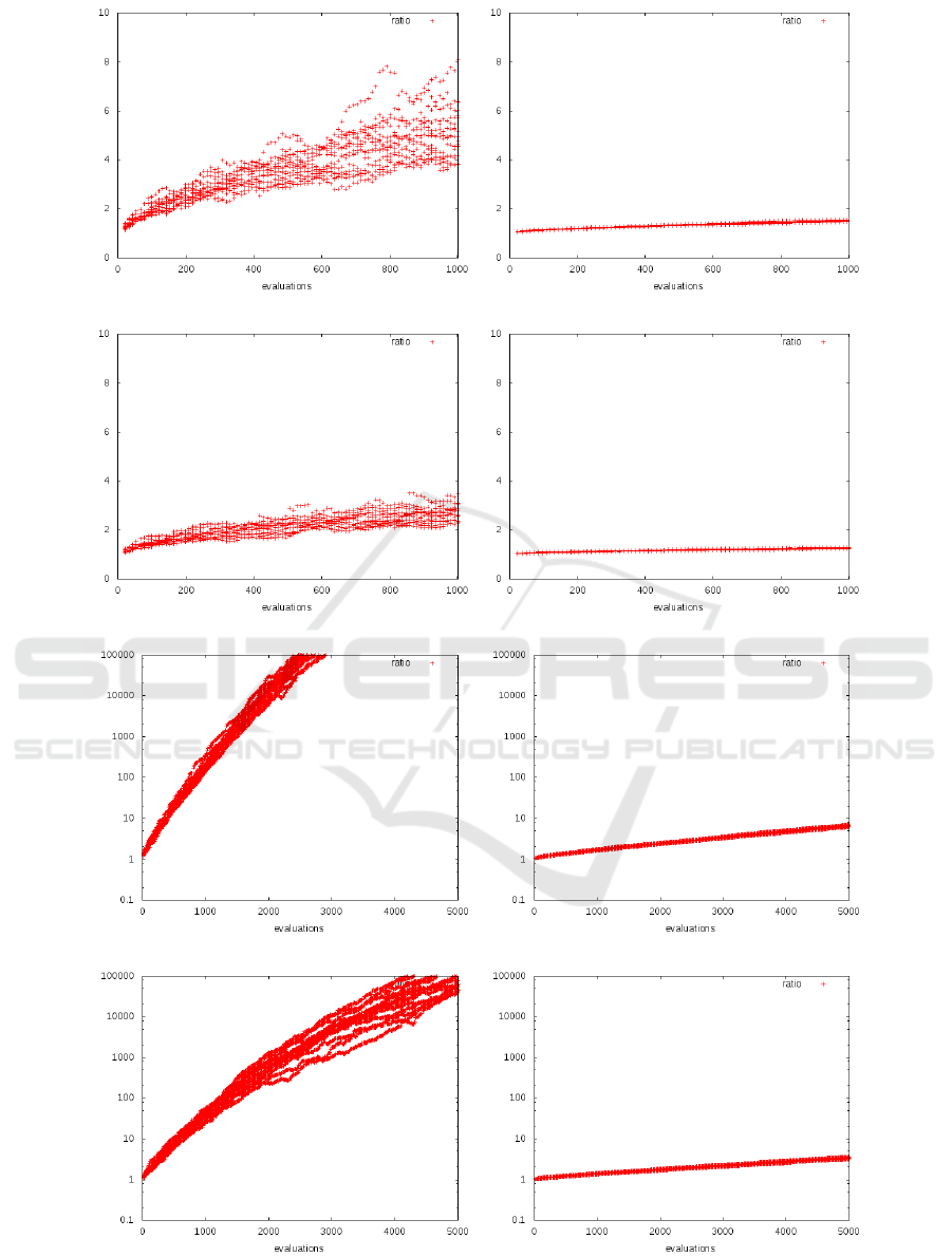
a) CMSA-ES, sphere, N = 10 b) CMSA-ES, sphere, N = 40
c) CC-ES, sphere, N = 10 d) CC-ES, sphere, N = 40
e) CMSA-ES, discus, N = 10 f) CMSA-ES, discus, N = 40
g) CC-ES, discus, N = 10 h) CC-ES, discus, N = 40
Figure 2: The development of the ratio of the largest to the smallest eigenvalue of the covariance on the sphere and the discus.
Shown are the results from 15runs per dimensionality.
Evolution Strategies and Covariance Matrix Adaptation - Investigating New Shrinkage Techniques
111

Table 1: Expected running time (ERT in number of function evaluations) divided by the respective best ERT measured during
BBOB-2009 in dimension 10. The ERT and in braces, as dispersion measure, the half difference between 90 and 10%-tile
of bootstrapped run lengths appear for each algorithm and target, the corresponding best ERT in the first row. The different
target ∆f -values are shown in the top row. #succ is the number of trials that reached the (final) target f
opt
+10
−8
. The median
number of conducted function evaluations is additionally given in italics, if the target in the last column was never reached.
10-D
∆ f
opt
1e1 1e0 1e-1 1e-2 1e-3 1e-5 1e-7 #succ
f1 22 23 23 23 23 23 23 15/15
CMSA 4.0(2) 8.6(3) 14(5) 19(3) 26(5) 38(6) 50(5) 15/15
CC-ES 3.7(2) 8.4(3) 13(3) 18(3) 23(3) 35(5) 45(3) 15/15
CI-ES 4.2(1) 9.3(4) 14(4) 19(5) 24(4) 34(6) 43(2) 15/15
Tou-ES4.2(2) 9.1(3) 15(4) 21(3) 27(4) 40(7) 54(11) 15/15
FS-ES 4.2(2) 10(2) 14(4) 19(2) 25(4) 37(5) 49(6) 15/15
∆ f
opt
1e1 1e0 1e-1 1e-2 1e-3 1e-5 1e-7 #succ
f2 187 190 191 191 193 194 195 15/15
CMSA 65(30) 85(23) 96(23) 105(22) 109(31) 113(27) 129(27) 15/15
CC-ES ∞ ∞ ∞ ∞ ∞ ∞ ∞ 2e5 0/15
CI-ES ∞ ∞ ∞ ∞ ∞ ∞ ∞ 2e5 0/15
Tou-ES496(217) 850(584) 1517(1640)1835(1954)1833(1007)2248(1961)2757(2246) 5/15
FS-ES 62(28) 90(26) 102(37) 110(25) 117(22) 125(31) 129(22) 15/15
∆ f
opt
1e1 1e0 1e-1 1e-2 1e-3 1e-5 1e-7 #succ
f5 20 20 20 20 20 20 20 15/15
CMSA 12(5) 17(6) 17(10) 17(9) 17(6) 17(11) 17(9) 15/15
CC-ES 18(13) 102(307) 104(305) 104(16) 104(16) 104(17) 104(601) 15/15
CI-ES 14(7) 19(12) 20(15) 20(10) 20(9) 20(13) 20(12) 15/15
Tou-ES12(11) 18(17) 19(8) 19(12) 19(4) 19(6) 19(32) 15/15
FS-ES 12(5) 16(7) 16(6) 16(7) 16(9) 16(8) 16(6) 15/15
∆ f
opt
1e1 1e0 1e-1 1e-2 1e-3 1e-5 1e-7 #succ
f6 412 623 826 1039 1292 1841 2370 15/15
CMSA 1.4(0.9) 3.3(4) 11(31) 14(6) 19(22) 25(28) 163(176) 6/15
CC-ES 1.2(0.3) 18(1) 68(39) 193(254) 1088(1315) ∞ ∞ 2e5 0/15
CI-ES 37(3) 60(42) 183(77) 219(358) 348(1037) 452(522) 1206(823) 1/15
Tou-ES 5.3(0.4) 89(113) 135(168) 138(64) 151(67) 369(200) ∞ 2e5 0/15
FS-ES 1.9(0.6) 3.3(2) 14(6) 19(21) 25(10) 37(45) 75(37) 11/15
∆ f
opt
1e1 1e0 1e-1 1e-2 1e-3 1e-5 1e-7 #succ
f7 172 1611 4195 5099 5141 5141 5389 15/15
CMSA 4.0(6) 26(16) 85(66) ∞ ∞ ∞ ∞ 2e5 0/15
CC-ES 2.1(3) 42(29) 338(306) ∞ ∞ ∞ ∞ 2e5 0/15
CI-ES 3.4(2) 34(34) 204(155) ∞ ∞ ∞ ∞ 2e5 0/15
Tou-ES3.2(5) 37(69) 323(155) ∞ ∞ ∞ ∞ 2e5 0/15
FS-ES 4.5(6) 78(33) 206(167) ∞ ∞ ∞ ∞ 2e5 0/15
∆ f
opt
1e1 1e0 1e-1 1e-2 1e-3 1e-5 1e-7 #succ
f8 326 921 1114 1217 1267 1315 1343 15/15
CMSA 3.3(2) 17(10) 18(9) 18(6) 18(6) 19(10) 19(9) 15/15
CC-ES 17(38) 378(428) 784(1249) 2310(1972) ∞ ∞ ∞ 2e5 0/15
CI-ES 75(163) 197(130) ∞ ∞ ∞ ∞ ∞ 2e5 0/15
Tou-ES11(17) 68(18) 72(30) 76(30) 77(39) 78(33) 79(33) 15/15
FS-ES 4.2(8) 17(13) 18(8) 17(5) 17(13) 18(3) 18(8) 15/15
∆ f
opt
1e1 1e0 1e-1 1e-2 1e-3 1e-5 1e-7 #succ
f9 200 648 857 993 1065 1138 1185 15/15
CMSA 2.3(2) 25(18) 24(3) 22(11) 22(11) 21(10) 21(4) 15/15
CC-ES 16(33) 2122(2603) ∞ ∞ ∞ ∞ ∞ 2e5 0/15
CI-ES 2.2(1) 323(319) ∞ ∞ ∞ ∞ ∞ 2e5 0/15
Tou-ES 4.8(10) 91(31) 86(44) 86(46) 84(36) 84(27) 83(23) 15/15
FS-ES 3.5(2) 19(13) 19(5) 18(9) 18(13) 18(4) 18(12) 15/15
∆ f
opt
1e1 1e0 1e-1 1e-2 1e-3 1e-5 1e-7 #succ
f10 1835 2172 2455 2728 2802 4543 4739 15/15
CMSA 6.5(3) 7.6(1) 7.7(3) 7.5(4) 7.6(3) 4.9(1) 4.9(2) 15/15
CC-ES ∞ ∞ ∞ ∞ ∞ ∞ ∞ 2e5 0/15
CI-ES ∞ ∞ ∞ ∞ ∞ ∞ ∞ 2e5 0/15
Tou-ES111(72) 301(192) 608(815) ∞ ∞ ∞ ∞ 2e5 0/15
FS-ES 5.7(2) 7.9(1) 7.7(2) 7.5(1) 7.9(1) 5.2(1) 5.3(1) 15/15
∆ f
opt
1e1 1e0 1e-1 1e-2 1e-3 1e-5 1e-7 #succ
f11 266 1041 2602 2954 3338 4092 4843 15/15
CMSA 14(3) 6.2(2) 3.2(1) 3.4(2) 3.5(1) 3.3(0.9) 3.0(2) 15/15
CC-ES 1.1e4(1e4) ∞ ∞ ∞ ∞ ∞ ∞ 2e5 0/15
CI-ES ∞ ∞ ∞ ∞ ∞ ∞ ∞ 2e5 0/15
Tou-ES152(258) 169(152) 150(143) 312(614) 277(312) 343(354) 596(1270) 1/15
FS-ES 16(5) 6.3(2) 3.2(0.9) 3.3(1) 3.3(1) 3.3(0.6) 3.0(0.6) 15/15
∆ f
opt
1e1 1e0 1e-1 1e-2 1e-3 1e-5 1e-7 #succ
f12 515 896 1240 1390 1569 3660 5154 15/15
CMSA 4.2(0.2) 10(6) 13(13) 15(13) 16(9) 8.8(5) 7.8(2) 15/15
CC-ES 11(18) 37(15) 68(142) 161(241) 572(444) ∞ ∞ 2e5 0/15
CI-ES 29(97) 615(669) 2258(4031) 2020(1655) ∞ ∞ ∞ 2e5 0/15
Tou-ES76(228) 177(170) 722(1674) 1016(1115) 910(970) 799(464) 569(378) 1/15
FS-ES 2.3(2) 10(12) 13(8) 15(8) 16(10) 10(5) 10(6) 15/15
∆ f
opt
1e1 1e0 1e-1 1e-2 1e-3 1e-5 1e-7 #succ
f13 387 596 797 1014 4587 6208 7779 15/15
CMSA 15(11) 19(34) 31(33) 58(115) 28(23) 89(114) 185(129) 2/15
CC-ES 19(36) 59(71) 186(311) 610(1661) 637(1243) ∞ ∞ 2e5 0/15
CI-ES 32(6) 57(118) 87(46) 229(245) 145(147) ∞ ∞ 2e5 0/15
Tou-ES22(45) 50(37) 117(68) 500(786) 307(262) ∞ ∞ 2e5 0/15
FS-ES 5.1(0.5) 23(32) 35(49) 66(52) 31(55) 98(128) 183(238) 2/15
∆ f
opt
1e1 1e0 1e-1 1e-2 1e-3 1e-5 1e-7 #succ
f14 37 98 133 205 392 687 4305 15/15
CMSA 1.1(1) 2.2(0.6) 2.8(0.5) 3.5(1) 4.3(0.5) 8.7(3) 4.8(3) 15/15
CC-ES 0.98(1) 2.4(1) 2.9(1) 3.6(2) 72(70) ∞ ∞ 2e5 0/15
CI-ES 1.2(0.9) 2.4(1) 2.9(1) 3.6(3) 24(6) ∞ ∞ 2e5 0/15
Tou-ES1.4(2) 2.7(0.5) 3.5(2) 5.4(2) 24(20) 241(169) 339(314) 2/15
FS-ES 1.4(1) 2.6(1) 3.0(1) 3.7(1) 4.5(1.0) 10(4) 4.5(2) 15/15
∆ f
opt
1e1 1e0 1e-1 1e-2 1e-3 1e-5 1e-7 #succ
f16 425 7029 15779 45669 51151 65798 71570 15/15
CMSA 1.0(0.7) 1.8(2) 13(14) 31(12) ∞ ∞ ∞ 2e5 0/15
CC-ES 1.1(2) 2.3(1) 43(35) ∞ ∞ ∞ ∞ 2e5 0/15
CI-ES 0.76(1.0) 19(14) 180(133) ∞ ∞ ∞ ∞ 2e5 0/15
Tou-ES1.2(1) 8.7(18) 179(139) ∞ ∞ ∞ ∞ 2e5 0/15
FS-ES 1.7(0.7) 0.55(0.7) 23(27) ∞ ∞ ∞ ∞ 2e5 0/15
∆ f
opt
1e1 1e0 1e-1 1e-2 1e-3 1e-5 1e-7 #succ
f17 26 429 2203 6329 9851 20190 26503 15/15
CMSA 0.71(0.4) 18(26) 23(44) 30(17) 140(86) ∞ ∞ 2e5 0/15
CC-ES 0.72(0.5) 20(12) 20(26) 39(114) 304(436) ∞ ∞ 2e5 0/15
CI-ES 1.2(0.5) 171(117) 182(227) ∞ ∞ ∞ ∞ 2e5 0/15
Tou-ES1.6(1) 52(43) 75(115) 141(174) ∞ ∞ ∞ 2e5 0/15
FS-ES 1.00(3) 26(29) 27(48) 77(107) 424(559) ∞ ∞ 2e5 0/22
∆ f
opt
1e1 1e0 1e-1 1e-2 1e-3 1e-5 1e-7 #succ
f18 238 836 7012 15928 27536 37234 42708 15/15
CMSA 68(47) 129(298) 124(54) ∞ ∞ ∞ ∞ 2e5 0/15
CC-ES 8.8(28) 38(71) 55(60) ∞ ∞ ∞ ∞ 2e5 0/15
CI-ES 3.3(17) 136(124) 124(235) ∞ ∞ ∞ ∞ 2e5 0/15
Tou-ES 8.5(1.0) 187(237) 211(135) ∞ ∞ ∞ ∞ 2e5 0/15
FS-ES 2.6(0.8) 98(79) 94(124) ∞ ∞ ∞ ∞ 2e5 0/15
∆ f
opt
1e1 1e0 1e-1 1e-2 1e-3 1e-5 1e-7 #succ
f20 32 15426 5.5e5 5.7e5 5.7e5 5.8e5 5.9e5 15/15
CMSA 1.9(1) 25(37) ∞ ∞ ∞ ∞ ∞ 2e5 0/15
CC-ES 1.9(1) 33(17) ∞ ∞ ∞ ∞ ∞ 2e5 0/15
CI-ES 2.1(1) 38(55) ∞ ∞ ∞ ∞ ∞ 2e5 0/15
Tou-ES1.8(1) 56(101) ∞ ∞ ∞ ∞ ∞ 2e5 0/15
FS-ES 1.5(0.7) 24(32) ∞ ∞ ∞ ∞ ∞ 2e5 0/15
∆ f
opt
1e1 1e0 1e-1 1e-2 1e-3 1e-5 1e-7 #succ
f21 130 2236 4392 4487 4618 5074 11329 8/15
CMSA 9.5(11) 23(24) 20(15) 20(20) 19(28) 17(40) 7.8(9) 12/15
CC-ES 33(54) 18(10) 13(18) 17(13) 16(10) 36(19) 35(49) 6/15
CI-ES 47(133) 109(268) 58(56) 57(92) 55(102) 50(50) 23(46) 8/15
Tou-ES50(232) 39(98) 32(76) 31(23) 30(44) 28(74) 14(6) 9/15
FS-ES 13(50) 16(27) 10(13) 9.4(13) 9.2(12) 8.4(6) 3.8(6) 15/15
∆ f
opt
1e1 1e0 1e-1 1e-2 1e-3 1e-5 1e-7 #succ
f22 98 2839 6353 6620 6798 8296 10351 6/15
CMSA 25(45) 6.3(9) 13(23) 12(16) 12(19) 10(14) 8.1(9) 13/15
CC-ES 48(63) 13(12) 23(21) 49(21) 133(238) ∞ ∞ 2e5 0/15
CI-ES 149(369) 29(72) 24(43) 25(26) 25(22) 30(48) ∞ 2e5 0/15
Tou-ES 61(132) 10(12) 17(14) 17(17) 17(22) 16(24) 14(19) 12/15
FS-ES 22(68) 14(22) 11(13) 11(20) 11(18) 9.0(5) 7.3(11) 13/15
Schwefel (id 20). In these cases, all strategies are un-
able to progress further than the first intermediate pre-
cision of 10
1
. Additionally, for the multi-modal func-
tions, 19 (Composite Griewank-Rosenbrock Func-
tion) and 23 (Katsuura), no strategy could reach 10
−1
.
The functions in question are removed from the ta-
bles.
To analyze the remaining functions, the four
groups of the test suite are taken into account. The
first class comprises the separable functions with id
1 to id 5. The three remaining functions, the sphere
(f1), the separable ellipsoidal function (f2), and the
linear slope (f5) differ in the degree of difficulty for
the strategies. All strategies do not show any prob-
ICAART 2016 - 8th International Conference on Agents and Artificial Intelligence
112

Table 2: Expected running time (ERT in number of function evaluations) divided by the respective best ERT measured during
BBOB-2009 in dimension 20. The ERT and in braces, as dispersion measure, the half difference between 90 and 10%-tile
of bootstrapped run lengths appear for each algorithm and target, the corresponding best ERT in the first row. The different
target ∆f -values are shown in the top row. #succ is the number of trials that reached the (final) target f
opt
+10
−8
. The median
number of conducted function evaluations is additionally given in italics, if the target in the last column was never reached.
20-D
∆ f
opt
1e1 1e0 1e-1 1e-2 1e-3 1e-5 1e-7 #succ
f1 43 43 43 43 43 43 43 15/15
CMSA 4.9(2) 10(0.9) 15(2) 19(2) 25(2) 34(2) 45(2) 15/15
CC-ES 4.7(1) 8.9(2) 14(1) 19(2) 23(2) 33(4) 42(3) 15/15
CI-ES 5.0(1) 10(1) 15(2) 19(2) 24(2) 34(2) 44(2) 15/15
Tou-ES5.1(0.9) 10(1) 14(2) 19(2) 25(3) 35(5) 46(4) 15/15
FS-ES 4.8(2) 10(1) 14(3) 19(2) 24(2) 34(3) 44(4) 15/15
∆ f
opt
1e1 1e0 1e-1 1e-2 1e-3 1e-5 1e-7 #succ
f2 385 386 387 388 390 391 393 15/15
CMSA 173(26) 240(36) 265(23) 273(41) 277(37) 285(28) 293(37) 15/15
CC-ES ∞ ∞ ∞ ∞ ∞ ∞ ∞ 4e5 0/15
CI-ES ∞ ∞ ∞ ∞ ∞ ∞ ∞ 4e5 0/15
Tou-ES ∞ ∞ ∞ ∞ ∞ ∞ ∞ 4e5 0/15
FS-ES 162(21) 224(70) 263(40) 278(28) 285(36) 296(19) 308(52) 15/15
∆ f
opt
1e1 1e0 1e-1 1e-2 1e-3 1e-5 1e-7 #succ
f5 41 41 41 41 41 41 41 15/15
CMSA 12(4) 15(7) 15(4) 15(7) 15(7) 15(5) 15(6) 15/15
CC-ES 13(7) 17(8) 18(7) 18(10) 18(7) 18(9) 18(10) 15/15
CI-ES 14(8) 18(7) 19(6) 19(7) 19(15) 19(22) 19(8) 15/15
Tou-ES11(3) 14(3) 14(5) 14(4) 14(4) 14(6) 14(4) 15/15
FS-ES 12(5) 14(4) 15(4) 15(4) 15(4) 15(7) 15(4) 15/15
∆ f
opt
1e1 1e0 1e-1 1e-2 1e-3 1e-5 1e-7 #succ
f6 1296 2343 3413 4255 5220 6728 8409 15/15
CMSA 1.5(0.4) 2.5(2) 4.6(2) 12(23) 34(15) 80(90) 331(393) 2/15
CC-ES 80(80) 471(640) 1643(1465) ∞ ∞ ∞ ∞ 4e5 0/15
CI-ES 29(232) 88(128) 108(177) 154(236) 144(230) 253(253) 206(187) 3/15
Tou-ES56(27) 275(515) ∞ ∞ ∞ ∞ ∞ 4e5 0/15
FS-ES 2.0(0.7) 3.9(4) 6.1(6) 19(9) 64(58) 265(357) ∞ 4e5 0/15
∆ f
opt
1e1 1e0 1e-1 1e-2 1e-3 1e-5 1e-7 #succ
f8 2039 3871 4040 4148 4219 4371 4484 15/15
CMSA 11(9) 30(3) 31(54) 31(8) 31(99) 31(6) 31(47) 13/15
CC-ES 2752(4660) ∞ ∞ ∞ ∞ ∞ ∞ 4e5 0/15
CI-ES 106(132) 727(1259) ∞ ∞ ∞ ∞ ∞ 4e5 0/15
Tou-ES 96(46) ∞ ∞ ∞ ∞ ∞ ∞ 4e5 0/15
FS-ES 13(6) 31(6) 33(52) 33(31) 33(53) 32(25) 32(44) 13/15
∆ f
opt
1e1 1e0 1e-1 1e-2 1e-3 1e-5 1e-7 #succ
f9 1716 3102 3277 3379 3455 3594 3727 15/15
CMSA 17(6) 40(63) 41(63) 41(91) 41(88) 40(31) 40(29) 13/15
CC-ES ∞ ∞ ∞ ∞ ∞ ∞ ∞ 4e5 0/15
CI-ES 158(161) ∞ ∞ ∞ ∞ ∞ ∞ 4e5 0/15
Tou-ES 88(32) 633(291) ∞ ∞ ∞ ∞ ∞ 4e5 0/15
FS-ES 17(7) 31(2) 33(4) 33(5) 33(32) 33(30) 32(2) 14/15
∆ f
opt
1e1 1e0 1e-1 1e-2 1e-3 1e-5 1e-7 #succ
f10 7413 8661 10735 13641 14920 17073 17476 15/15
CMSA 10(3) 11(2) 9.2(2) 7.8(2) 7.3(1) 6.7(0.8) 6.8(1.0) 15/15
CC-ES ∞ ∞ ∞ ∞ ∞ ∞ ∞ 4e5 0/15
CI-ES ∞ ∞ ∞ ∞ ∞ ∞ ∞ 4e5 0/15
Tou-ES796(445) ∞ ∞ ∞ ∞ ∞ ∞ 4e5 0/15
FS-ES 8.3(3) 10(1) 8.4(2) 7.0(1) 6.8(0.7) 6.2(0.5) 6.3(0.6) 15/15
∆ f
opt
1e1 1e0 1e-1 1e-2 1e-3 1e-5 1e-7 #succ
f11 1002 2228 6278 8586 9762 12285 14831 15/15
CMSA 12(2) 7.5(0.9) 3.1(0.1) 2.6(0.5) 2.6(0.4) 2.5(0.6) 2.5(0.4) 15/15
CC-ES ∞ ∞ ∞ ∞ ∞ ∞ ∞ 4e5 0/15
CI-ES ∞ ∞ ∞ ∞ ∞ ∞ ∞ 4e5 0/15
Tou-ES2831(3585) ∞ ∞ ∞ ∞ ∞ ∞ 4e5 0/15
FS-ES 12(2) 6.7(0.8) 2.7(0.6) 2.4(0.6) 2.5(0.4) 2.4(0.6) 2.3(0.4) 15/15
∆ f
opt
1e1 1e0 1e-1 1e-2 1e-3 1e-5 1e-7 #succ
f12 1042 1938 2740 3156 4140 12407 13827 15/15
CMSA 2.5(0.1) 10(9) 13(8) 15(6) 14(5) 5.9(2) 6.2(2) 15/15
CC-ES 97(480) 569(568) 2045(2299) 1775(887) ∞ ∞ ∞ 4e5 0/15
CI-ES 60(96) 182(206) 585(365) 1775(3993) ∞ ∞ ∞ 4e5 0/15
Tou-ES97(192) 137(139) 315(357) 1775(1901) ∞ ∞ ∞ 4e5 0/15
FS-ES 4.9(0.2) 12(11) 14(10) 16(12) 15(7) 6.3(3) 6.5(3) 15/15
∆ f
opt
1e1 1e0 1e-1 1e-2 1e-3 1e-5 1e-7 #succ
f13 652 2021 2751 3507 18749 24455 30201 15/15
CMSA 156(154) 545(594) 2037(1600) ∞ ∞ ∞ ∞ 4e5 0/15
CC-ES 97(307) 397(495) 2037(2181) ∞ ∞ ∞ ∞ 4e5 0/15
CI-ES 97(155) 397(396) 584(763) ∞ ∞ ∞ ∞ 4e5 0/15
Tou-ES309(460) 545(742) 947(1309) ∞ ∞ ∞ ∞ 4e5 0/15
FS-ES 97(460) 298(396) 2037(2509) ∞ ∞ ∞ ∞ 4e5 0/15
∆ f
opt
1e1 1e0 1e-1 1e-2 1e-3 1e-5 1e-7 #succ
f14 75 239 304 451 932 1648 15661 15/15
CMSA 1.8(0.9) 1.9(0.7) 2.5(0.5) 3.2(0.6) 5.2(0.8) 11(3) 4.2(1) 15/15
CC-ES 1.8(0.4) 1.9(0.6) 2.4(0.6) 3.1(0.6) ∞ ∞ ∞ 4e5 0/15
CI-ES 1.8(0.6) 1.8(0.4) 2.4(0.5) 3.4(1.0) 23(4) ∞ ∞ 4e5 0/15
Tou-ES1.5(0.4) 1.7(0.5) 2.3(0.7) 3.5(0.7) 27(21) ∞ ∞ 4e5 0/15
FS-ES 2.0(1) 1.9(0.5) 2.4(0.5) 3.2(0.8) 4.8(0.3) 12(2) 3.9(0.5) 15/15
∆ f
opt
1e1 1e0 1e-1 1e-2 1e-3 1e-5 1e-7 #succ
f16 1384 27265 77015 1.4e5 1.9e5 2.0e5 2.2e5 15/15
CMSA 22(145) 95(106) ∞ ∞ ∞ ∞ ∞ 4e5 0/15
CC-ES 45(145) ∞ ∞ ∞ ∞ ∞ ∞ 4e5 0/15
CI-ES 45(217) 95(114) ∞ ∞ ∞ ∞ ∞ 4e5 0/15
Tou-ES21(0.9) 205(308) ∞ ∞ ∞ ∞ ∞ 4e5 0/15
FS-ES 45(218) ∞ ∞ ∞ ∞ ∞ ∞ 4e5 0/15
∆ f
opt
1e1 1e0 1e-1 1e-2 1e-3 1e-5 1e-7 #succ
f17 63 1030 4005 12242 30677 56288 80472 15/15
CMSA 0.93(0.9) 196(97) ∞ ∞ ∞ ∞ ∞ 4e5 0/15
CC-ES 1.3(0.5) 341(194) 650(949) ∞ ∞ ∞ ∞ 4e5 0/15
CI-ES 1.1(0.8) 445(486) ∞ ∞ ∞ ∞ ∞ 4e5 0/15
Tou-ES1.2(0.6) 778(486) 1399(1473) ∞ ∞ ∞ ∞ 4e5 0/15
FS-ES 1.7(3) 260(583) ∞ ∞ ∞ ∞ ∞ 4e5 0/15
∆ f
opt
1e1 1e0 1e-1 1e-2 1e-3 1e-5 1e-7 #succ
f18 621 3972 19561 28555 67569 1.3e5 1.5e5 15/15
CMSA 48(0.9) ∞ ∞ ∞ ∞ ∞ ∞ 4e5 0/15
CC-ES 1.3(1) 277(453) ∞ ∞ ∞ ∞ ∞ 4e5 0/15
CI-ES 47(0.9) 1410(2946) ∞ ∞ ∞ ∞ ∞ 4e5 0/15
Tou-ES 1.3(1) 655(579) ∞ ∞ ∞ ∞ ∞ 4e5 0/15
FS-ES 101(484) 655(529) ∞ ∞ ∞ ∞ ∞ 4e5 0/15
∆ f
opt
1e1 1e0 1e-1 1e-2 1e-3 1e-5 1e-7 #succ
f21 561 6541 14103 14318 14643 15567 17589 15/15
CMSA 179(178) 245(138) 113(113) 112(70) 109(109) 103(128) 91(85) 3/15
CC-ES 357(713) 168(122) 113(50) 112(105) 109(184) 103(218) 91(91) 3/15
CI-ES 357(1247) 398(413) 184(128) 182(321) 178(96) 167(212) 148(159) 2/15
Tou-ES179(356) 122(306) 78(135) 77(77) 75(137) 71(71) 63(159) 4/15
FS-ES 179(178) 122(61) 78(113) 77(77) 75(41) 71(96) 63(57) 4/15
∆ f
opt
1e1 1e0 1e-1 1e-2 1e-3 1e-5 1e-7 #succ
f22 467 5580 23491 24163 24948 26847 1.3e5 12/15
CMSA 572(1500) 287(215) ∞ ∞ ∞ ∞ ∞ 4e5 0/15
CC-ES 312(1071) 108(125) ∞ ∞ ∞ ∞ ∞ 4e5 0/15
CI-ES 980(1285) 466(627) ∞ ∞ ∞ ∞ ∞ 4e5 0/15
Tou-ES572(857) 287(197) 239(315) 232(128) 225(341) 211(183) 43(36) 1/15
FS-ES 751(1286) 466(502) ∞ ∞ ∞ ∞ ∞ 4e5 0/15
lems on the sphere or on the slope. Here, several
shrinkage variants surpass the original version. The
more difficult ellipsoidal function, however, cannot
be solved by the CC-ES, the CI-ES, and for N =20
and N =40 by the Tou-ES. Interestingly, the FS-ES
achieves successful runs for all search space dimen-
sionalities. Its performance is similar to the origi-
nal CMSA-ES. However, the latter shows the better
performance in many cases. Two effects may play
a role. The ellipsoidal function, defined by f (x)=
∑
N
i=1
10
6(i−1)/(N−1)
x
2
i
, is not solved well by ESs with
covariance matrices treating all directions with the
same weight. The matrix used in the basis transforma-
tion may not be sufficient to provide the variability re-
quired if combined with structures that are restrictive.
The structures supplied by the CC-ES and the CI-ES
may be too regular for the ES to be able to adapt with
the necessary velocity. The failure of the Tou-ES to
achieve the final precision target may be due to the
shrinkage intensity since this is the only point where
it differs from the FS-ES. In future research, exper-
iments will be performed that use lower shrinkage
intensities. Also the interaction with the parameter
c
τ
will be taken into account and investigated more
Evolution Strategies and Covariance Matrix Adaptation - Investigating New Shrinkage Techniques
113

Table 3: Expected running time (ERT in number of function evaluations) divided by the respective best ERT measured during
BBOB-2009 in dimension 40. The ERT and in braces, as dispersion measure, the half difference between 90 and 10%-tile
of bootstrapped run lengths appear for each algorithm and target, the corresponding best ERT in the first row. The different
target ∆f -values are shown in the top row. #succ is the number of trials that reached the (final) target f
opt
+10
−8
. The median
number of conducted function evaluations is additionally given in italics, if the target in the last column was never reached.
40-D
∆ f
opt
1e1 1e0 1e-1 1e-2 1e-3 1e-5 1e-7 #succ
f1 83 83 83 83 83 83 83 30/30
CMSA 5.8(1) 10(0.9) 14(2) 18(1) 23(2) 32(3) 40(2) 15/15
CC-ES 5.1(0.9) 9.3(1) 14(2) 18(1) 23(1) 31(3) 40(3) 15/15
CI-ES 5.5(1) 10(1) 14(2) 18(2) 23(2) 31(2) 40(1) 15/15
Tou-ES6.3(2) 11(2) 15(0.8) 19(2) 24(2) 33(1) 42(3) 15/15
FS-ES 5.4(0.7) 10(2) 14(2) 18(2) 22(2) 31(2) 40(2) 15/15
∆ f
opt
1e1 1e0 1e-1 1e-2 1e-3 1e-5 1e-7 #succ
f2 796 797 799 799 800 802 804 15/15
CMSA 367(65) 541(94) 665(90) 736(79) 786(92) 817(59) 837(49) 15/15
CC-ES ∞ ∞ ∞ ∞ ∞ ∞ ∞ 8e5 0/15
CI-ES ∞ ∞ ∞ ∞ ∞ ∞ ∞ 8e5 0/15
Tou-ES ∞ ∞ ∞ ∞ ∞ ∞ ∞ 8e5 0/15
FS-ES 391(124) 559(130) 651(93) 718(168) 787(81) 823(46) 837(80) 15/15
∆ f
opt
1e1 1e0 1e-1 1e-2 1e-3 1e-5 1e-7 #succ
f5 98 116 120 121 121 121 121 15/15
CMSA 11(5) 12(4) 12(2) 12(8) 12(4) 12(4) 12(6) 15/15
CC-ES 11(7) 11(9) 11(11) 11(6) 11(8) 11(5) 11(7) 15/15
CI-ES 10(4) 11(6) 11(6) 11(6) 11(6) 11(5) 11(5) 15/15
Tou-ES 9.3(3) 10(2) 10(2) 10(2) 10(3) 10(3) 10(3) 15/15
FS-ES 8.4(2) 8.3(2) 8.2(2) 8.2(2) 8.2(2) 8.2(2) 8.2(1) 15/15
∆ f
opt
1e1 1e0 1e-1 1e-2 1e-3 1e-5 1e-7 #succ
f6 3507 5523 7168 9470 11538 15007 19222 15/15
CMSA 3.9(2) 10(5) 22(18) 87(86) 312(258) ∞ ∞ 8e5 0/15
CC-ES 206(229) 948(904) ∞ ∞ ∞ ∞ ∞ 8e5 0/15
CI-ES 285(171) 946(905) 1568(2093) 1191(1478) 1033(832) ∞ ∞ 8e5 0/15
Tou-ES645(684) ∞ ∞ ∞ ∞ ∞ ∞ 8e5 0/15
FS-ES 4.0(2) 10(12) 28(33) 51(37) 142(113) ∞ ∞ 8e5 0/15
∆ f
opt
1e1 1e0 1e-1 1e-2 1e-3 1e-5 1e-7 #succ
f8 7080 10655 11012 11265 11430 11701 11969 15/15
CMSA 30(12) 35(11) 36(28) 37(10) 37(90) 37(9) 36(26) 14/15
CC-ES ∞ ∞ ∞ ∞ ∞ ∞ ∞ 8e5 0/15
CI-ES 810(831) 1117(657) ∞ ∞ ∞ ∞ ∞ 8e5 0/15
Tou-ES1665(3051) ∞ ∞ ∞ ∞ ∞ ∞ 8e5 0/15
FS-ES 33(17) 37(17) 38(14) 38(9) 38(10) 38(14) 38(8) 14/15
∆ f
opt
1e1 1e0 1e-1 1e-2 1e-3 1e-5 1e-7 #succ
f9 6122 12982 13300 13496 13651 13909 14142 15/15
CMSA 43(9) 38(36) 40(32) 40(32) 40(7) 40(18) 40(30) 13/15
CC-ES ∞ ∞ ∞ ∞ ∞ ∞ ∞ 8e5 0/15
CI-ES ∞ ∞ ∞ ∞ ∞ ∞ ∞ 8e5 0/15
Tou-ES ∞ ∞ ∞ ∞ ∞ ∞ ∞ 8e5 0/15
FS-ES 43(9) 38(48) 39(32) 39(6) 39(32) 39(32) 39(17) 13/15
∆ f
opt
1e1 1e0 1e-1 1e-2 1e-3 1e-5 1e-7 #succ
f10 25890 30368 36796 51579 56007 65128 70824 15/15
CMSA 11(2) 14(4) 14(1) 11(1) 11(0.6) 10(0.6) 9.4(0.6) 15/15
CC-ES ∞ ∞ ∞ ∞ ∞ ∞ ∞ 8e5 0/15
CI-ES ∞ ∞ ∞ ∞ ∞ ∞ ∞ 8e5 0/15
Tou-ES ∞ ∞ ∞ ∞ ∞ ∞ ∞ 8e5 0/15
FS-ES 12(3) 14(1) 14(1) 11(1) 11(0.9) 10(0.5) 9.3(0.5) 15/15
∆ f
opt
1e1 1e0 1e-1 1e-2 1e-3 1e-5 1e-7 #succ
f11 2368 4855 11681 25315 29749 38949 48211 15/15
CMSA 16(1) 9.2(0.6) 4.2(0.5) 2.2(0.3) 2.0(0.2) 1.8(0.4) 1.6(0.3) 15/15
CC-ES ∞ ∞ ∞ ∞ ∞ ∞ ∞ 8e5 0/15
CI-ES ∞ ∞ ∞ ∞ ∞ ∞ ∞ 8e5 0/15
Tou-ES ∞ ∞ ∞ ∞ ∞ ∞ ∞ 8e5 0/15
FS-ES 16(2) 9.3(0.9) 4.3(0.6) 2.2(0.4) 2.0(0.2) 1.8(0.2) 1.6(0.3) 15/15
∆ f
opt
1e1 1e0 1e-1 1e-2 1e-3 1e-5 1e-7 #succ
f12 4169 7452 9174 10751 13146 22758 25192 15/15
CMSA 5.0(3) 7.8(9) 10(7) 11(7) 11(4) 7.6(2) 7.7(2) 15/15
CC-ES 49(48) 296(537) ∞ ∞ ∞ ∞ ∞ 8e5 0/15
CI-ES 97(240) 698(537) ∞ ∞ ∞ ∞ ∞ 8e5 0/15
Tou-ES28(48) 94(54) 567(981) ∞ ∞ ∞ ∞ 8e5 0/15
FS-ES 4.6(8) 10(8) 12(8) 12(4) 12(6) 8.1(2) 8.2(2) 15/15
∆ f
opt
1e1 1e0 1e-1 1e-2 1e-3 1e-5 1e-7 #succ
f13 2029 6916 8734 11861 71936 98467 1.2e5 15/15
CMSA 145(197) 102(260) 1283(710) ∞ ∞ ∞ ∞ 8e5 0/15
CC-ES 145(99) 174(174) 596(1214) ∞ ∞ ∞ ∞ 8e5 0/15
CI-ES 199(493) 174(145) 596(870) 945(1872) 156(158) ∞ ∞ 8e5 0/15
Tou-ES 62(197) 102(174) 596(366) 945(759) ∞ ∞ ∞ 8e5 0/15
FS-ES 62(99) 133(145) 596(733) 439(742) 156(259) ∞ ∞ 8e5 0/15
∆ f
opt
1e1 1e0 1e-1 1e-2 1e-3 1e-5 1e-7 #succ
f14 304 616 777 1105 2207 4825 57711 15/15
CMSA 1.2(0.4) 1.5(0.3) 1.9(0.2) 2.9(0.6) 6.2(0.8) 15(2) 4.6(0.5) 15/15
CC-ES 1.2(0.3) 1.6(0.6) 1.9(0.5) 2.9(0.7) ∞ ∞ ∞ 8e5 0/15
CI-ES 1.3(0.2) 1.6(0.2) 1.9(0.2) 3.1(0.9) 31(5) ∞ ∞ 8e5 0/15
Tou-ES1.3(0.4) 1.6(0.3) 2.0(0.3) 3.1(0.5) 32(5) ∞ ∞ 8e5 0/15
FS-ES 1.4(0.4) 1.7(0.7) 2.0(0.4) 2.9(0.3) 6.4(0.5) 16(3) 4.4(0.7) 15/15
∆ f
opt
1e1 1e0 1e-1 1e-2 1e-3 1e-5 1e-7 #succ
f17 399 4220 14158 34948 51958 1.3e5 2.7e5 14/15
CMSA 0.48(0.7) 1233(1517) ∞ ∞ ∞ ∞ ∞ 8e5 0/15
CC-ES 0.40(0.5)
↓3
759(758) ∞ ∞ ∞ ∞ ∞ 8e5 0/15
CI-ES 0.38(0.4)
↓4
759(332) ∞ ∞ ∞ ∞ ∞ 8e5 0/15
Tou-ES0.42(0.5)
↓2
759(1280) ∞ ∞ ∞ ∞ ∞ 8e5 0/15
FS-ES 0.55(0.7) 759(711) ∞ ∞ ∞ ∞ ∞ 8e5 0/15
∆ f
opt
1e1 1e0 1e-1 1e-2 1e-3 1e-5 1e-7 #succ
f21 1044 21144 1.0e5 1.0e5 1.0e5 1.0e5 1.0e5 26/30
CMSA 55(192) 104(85) 32(26) 32(26) 32(28) 31(22) 31(20) 3/15
CC-ES 192(767) 530(766) ∞ ∞ ∞ ∞ ∞ 8e5 0/15
CI-ES 512(575) 151(255) 52(77) 52(34) 51(97) 51(29) 51(61) 2/15
Tou-ES192(767) 246(568) ∞ ∞ ∞ ∞ ∞ 8e5 0/15
FS-ES 384(575) 530(416) 111(42) 111(103) 111(122) 110(135) 109(121) 1/15
∆ f
opt
1e1 1e0 1e-1 1e-2 1e-3 1e-5 1e-7 #succ
f22 3090 35442 6.5e5 6.5e5 6.5e5 6.5e5 6.5e5 8/30
CMSA 65(129) 34(51) ∞ ∞ ∞ ∞ ∞ 8e5 0/15
CC-ES 94(194) 45(135) ∞ ∞ ∞ ∞ ∞ 8e5 0/15
CI-ES 40(65) 45(34) ∞ ∞ ∞ ∞ ∞ 8e5 0/15
Tou-ES 65(130) 45(68) 17(18) 17(27) 17(24) 17(20) 18(19) 1/15
FS-ES 296(647) 147(226) ∞ ∞ ∞ ∞ ∞ 8e5 0/15
closely. Since the learning rate approaches infinity for
the typical µN ratios and increasing dimensionalities,
the influence of the sample covariance lessens. Regu-
larizing the covariance matrix may therefore be more
important for smaller to medium search space dimen-
sionalities. Concerning the question whether shrink-
age improves the performance, no clear answer can be
provided for the group of separable functions since
the ellipsoidal function apparently requires a faster
adaptation than the current versions supply.
The second group of functions consists of the at-
tractive sector function (id 6), the step ellipsoidal
function (id 7), the original Rosenbrock function (id
8), and a rotated Rosenbrock function (id 9). These
functions have low to moderate conditioning. The
sector function is difficult to solve for all strategies.
For N =40, no ES is able to reach the final precision
target with the number of evaluations allowed. For
N =20, successful runs were recorded for the CMSA-
ES and the CI-ES but only for a few cases, i.e., two or
three. Therefore, the question arises whether initial-
ization effects may have played a role and a compar-
ison is not attempted. For N =10, the FS-ES reaches
the final target precision of 10
−8
in eleven of 15 runs,
a result not mirrowed by the other strategies. Con-
cerning the Rosenbrock functions (f8 and f9), the
CMSA-ES and the FS-ES perform best, with the latter
resulting in lower ERT values on the rotated version
and the former on the original (with the exception of
N =10 where the shrinkage version surpasses the orig-
inal). Thus, the FS-ES may be preferable in the case
of the second group at least for smaller dimensional-
ICAART 2016 - 8th International Conference on Agents and Artificial Intelligence
114

ities. However, more experiments should be carried
out.
Functions with high conditioning constitute the
next group. The ellipsoidal function (f10), the dis-
cus (f11), the bent cigar (f12), the sharp ridge (f13),
and the different powers function (f14). Here, simi-
lar behaviors can be observed for the CMSA-ES and
the FS-ES with no clear advantage for either variant.
Both are able to reach the final target precision on the
functions with the exception of the sharp ridge where
only two successful runs are recorded for N =10 in
both cases. Again, these may be due to initialization
effects and should be treated therefore with care.
In the case of the multi-modal functions (ids 15-
24), all ESs encounter problems. Only for the two
Gallagher’s problems (id 21 and id 22) successes are
recorded. Here, the CMSA-ES and the versions that
use the diagonal elements of the sample covariance as
shrinkage target show the best results. The FS-ES ap-
pears to be a good choice for N =10. For N =20 and
N =40, only a few runs of all ESs reach the final tar-
get precision. Therefore, a comparison for the higher-
dimensional search spaces is difficult and is not car-
ried out in this paper. We will conduct further exper-
iments with a higher setting for the maximal number
of fitness evaluations in future work.
6 CONCLUSIONS
Evolution strategies rely on mutation as their main
search operator. This necessitates control and adap-
tation mechanisms. This paper considered the covari-
ance matrix adaptation together with self-adaptation.
Here, as for other approaches, the sample covariance
plays an important role. This estimate should be
treated with care, however, since it may not be reliable
in all cases. This holds especially if the sample size is
small with respect to the search space dimensionality
and therefore for most application cases of evolution
strategies. The paper provided an experimental anal-
ysis of shrinkage operators, an approach introduced
in statistics for correcting the sample covariance. The
covariance is shrunk towards a target and thus “cor-
rected”. The choice of the target and the combination
weight, the shrinkage intensity, are crucial. Since the
functions to be optimized may assume various struc-
tures, the approach must remain sufficiently adapt-
able. To achieve this, we considered a transformation
of the original search space. The experimental anal-
ysis took several shrinkage targets into account us-
ing the intensity settings of the original publications.
Pending further experiments that shall provide more
information regarding the shrinkage intensity which
may have interfered with the findings, shrinkage tar-
gets in the transformed space that use a diagonal ma-
trix consisting of the different entries of the trans-
formed sample covariance appear as the best choices.
Since the original covariance matrix adaptation per-
forms a further type of shrinkage which lessens the
influence of the sample covariance when the search
space dimensionality increases, effects may be more
pronounced for midsize dimensionalities. Future re-
search will focus on the shrinkage intensity and its
interaction with the covariance matrix adaptation.
REFERENCES
Beyer, H.-G. and Meyer-Nieberg, S. (2006). Self-adaptation
of evolution strategies under noisy fitness evalua-
tions. Genetic Programming and Evolvable Machines,
7(4):295–328.
Beyer, H.-G. and Sendhoff, B. (2008). Covariance matrix
adaptation revisited - the CMSA evolution strategy -.
In Rudolph, G. et al., editors, PPSN, volume 5199 of
Lecture Notes in Computer Science, pages 123–132.
Springer.
Chen, X., Wang, Z., and McKeown, M. (2012). Shrinkage-
to-tapering estimation of large covariance matri-
ces. Signal Processing, IEEE Transactions on,
60(11):5640–5656.
Chen, Y., Wiesel, A., Eldar, Y. C., and Hero, A. O.
(2010). Shrinkage algorithms for MMSE covariance
estimation. IEEE Transactions on Signal Processing,
58(10):5016–5029.
Dong, W. and Yao, X. (2007). Covariance matrix repair-
ing in gaussian based EDAs. In Evolutionary Com-
putation, 2007. CEC 2007. IEEE Congress on, pages
415–422.
Finck, S., Hansen, N., Ros, R., and Auger, A. (2010).
Real-parameter black-box optimization benchmark-
ing 2010: Presentation of the noiseless functions.
Technical report, Institute National de Recherche en
Informatique et Automatique. 2009/22.
Fisher, T. J. and Sun, X. (2011). Improved Stein-type
shrinkage estimators for the high-dimensional mul-
tivariate normal covariance matrix. Computational
Statistics & Data Analysis, 55(5):1909 – 1918.
Hansen, N. (2006). The CMA evolution strategy: A com-
paring review. In Lozano, J. et al., editors, To-
wards a new evolutionary computation. Advances in
estimation of distribution algorithms, pages 75–102.
Springer.
Hansen, N. (2008). Adaptive encoding: How to render
search coordinate system invariant. In Rudolph, G.,
Jansen, T., Beume, N., Lucas, S., and Poloni, C., edi-
tors, Parallel Problem Solving from Nature PPSN X,
volume 5199 of Lecture Notes in Computer Science,
pages 205–214. Springer Berlin Heidelberg.
Hansen, N., Auger, A., Finck, S., and Ros, R. (2012).
Real-parameter black-box optimization benchmark-
Evolution Strategies and Covariance Matrix Adaptation - Investigating New Shrinkage Techniques
115

ing 2012: Experimental setup. Technical report, IN-
RIA.
Hansen, N., Auger, A., Ros, R., Finck, S., and Po
ˇ
s
´
ık, P.
(2010). Comparing results of 31 algorithms from the
black-box optimization benchmarking BBOB-2009.
In Proceedings of the 12th annual conference com-
panion on Genetic and evolutionary computation,
GECCO ’10, pages 1689–1696, New York, NY, USA.
ACM.
Kramer, O. (2015). Evolution strategies with Ledoit-Wolf
covariance matrix estimation. In 2015 IEEE Congress
on Evolutionary Computation (IEEE CEC).
Ledoit, O. and Wolf, M. (2003). Improved estimation of the
covariance matrix of stock returns with an application
to portfolio selection. Journal of Empirical Finance,
10(5):603–621.
Ledoit, O. and Wolf, M. (2004a). Honey, I shrunk the sam-
ple covariance matrix. The Journal of Portfolio Man-
agement, 30(4):110–119.
Ledoit, O. and Wolf, M. (2004b). A well-conditioned
estimator for large dimensional covariance matrices.
Journal of Multivariate Analysis Archive, 88(2):265–
411.
Ledoit, O. and Wolf, M. (2012). Non-linear shrinkage esti-
mation of large dimensional covariance matrices. The
Annals of Statistics, 40(2):1024–1060.
Ledoit, O. and Wolf, M. (2014). Nonlinear shrinkage of the
covariance matrix for portfolio selection: Markowitz
meets goldilocks. Available at SSRN 2383361.
Meyer-Nieberg, S. and Beyer, H.-G. (2005). On the anal-
ysis of self-adaptive recombination strategies: First
results. In McKay, B. et al., editors, Proc. 2005
Congress on Evolutionary Computation (CEC’05),
Edinburgh, UK, pages 2341–2348, Piscataway NJ.
IEEE Press.
Meyer-Nieberg, S. and Beyer, H.-G. (2007). Self-adaptation
in evolutionary algorithms. In Lobo, F., Lima, C., and
Michalewicz, Z., editors, Parameter Setting in Evo-
lutionary Algorithms, pages 47–76. Springer Verlag,
Heidelberg.
Meyer-Nieberg, S. and Kropat, E. (2014). Adapting the
covariance in evolution strategies. In Proceedings of
ICORES 2014, pages 89–99. SCITEPRESS.
Meyer-Nieberg, S. and Kropat, E. (2015a). A new look at
the covariance matrix estimation in evolution strate-
gies. In Pinson, E., Valente, F., and Vitoriano, B.,
editors, Operations Research and Enterprise Systems,
volume 509 of Communications in Computer and In-
formation Science, pages 157–172. Springer Interna-
tional Publishing.
Meyer-Nieberg, S. and Kropat, E. (2015b). Small popu-
lations, high-dimensional spaces: Sparse covariance
matrix adaptation. In Computer Science and Informa-
tion Systems (FedCSIS), 2015 Federated Conference
on, pages 525–535.
Meyer-Nieberg, S. and Kropat, E. (2015c). Sparse covari-
ance matrix adaptation techniques for evolution strate-
gies. In Bramer, M. and Petridis, M., editors, Research
and Development in Intelligent Systems XXXII, pages
5–21. Springer International Publishing.
Pourahmadi, M. (2013). High-Dimensional Covariance Es-
timation: With High-Dimensional Data. John Wiley
& Sons.
Rechenberg, I. (1973). Evolutionsstrategie: Optimierung
technischer Systeme nach Prinzipien der biologischen
Evolution. Frommann-Holzboog Verlag, Stuttgart.
Sch
¨
affer, J. and Strimmer, K. (2005). A shrinkage approach
to large-scale covariance matrix estimation and impli-
cations for functional genomics,. Statistical Applica-
tions in Genetics and Molecular Biology, 4(1):Article
32.
Schwefel, H.-P. (1981). Numerical Optimization of Com-
puter Models. Wiley, Chichester.
Stein, C. (1956). Inadmissibility of the usual estimator for
the mean of a multivariate distribution. In Proc. 3rd
Berkeley Symp. Math. Statist. Prob. 1, pages 197–206.
Berkeley, CA.
Stein, C. (1975). Estimation of a covariance matrix. In Rietz
Lecture, 39th Annual Meeting. IMS, Atlanta, GA.
Thomaz, C. E., Gillies, D., and Feitosa, R. (2004). A new
covariance estimate for bayesian classifiers in biomet-
ric recognition. Circuits and Systems for Video Tech-
nology, IEEE Transactions on, 14(2):214–223.
Tong, T., Wang, C., and Wang, Y. (2014). Estimation of
variances and covariances for high-dimensional data:
a selective review. Wiley Interdisciplinary Reviews:
Computational Statistics, 6(4):255–264.
Touloumis, A. (2015). Nonparametric Stein-type shrink-
age covariance matrix estimators in high-dimensional
settings. Computational Statistics & Data Analysis,
83:251–261.
ICAART 2016 - 8th International Conference on Agents and Artificial Intelligence
116
