Strategies for Phylogenetic Reconstruction

For the Maximum Parsimony Problem

Karla E. Vazquez-Ortiz, Jean-Michel Richer and David Lesaint

LERIA, University of Angers, 2 Boulevard Lavoisier 49045, Angers Cedex 01, France

Keywords:

Phylogenetic Reconstruction, Maximum Parsimony, GPU, Simulated Annealing, Path-relinking.

Abstract:

The phylogenetic reconstruction is considered a central underpinning of diverse ﬁeld of biology like: ecology,

molecular biology and physiology. The main example is modeling patterns and processes of evolution. Ma-

ximum Parsimony (MP) is an important approach to solve the phylogenetic reconstruction by minimizing the

total number of genetic transformations, under this approach different metaheuristics have been implemented

like tabu search, genetic and memetic algorithms to cope with the combinatorial nature of the problem. In

this paper we review different strategies that could be added to existing implementations to improve their efﬁ-

ciency and accuracy. First we present two different techniques to evaluate the objective function by using CPU

and GPU technology, then we show a Path-Relinking implementation to compare tree topologies and ﬁnally

we introduces the application of these techniques in a Simulated Annealing algorithm looking for an optimal

solution.

1 INTRODUCTION

According to the scientiﬁc community of biology,

nowadays there are about 5 to 100 millions species of

organisms living on Earth. Phylogeny is the univer-

sal proposition accepted that suggests all organisms

on Earth are genetically related, and the genealogical

relationships of living things can be represented by a

vast evolutionary tree called phylogenetic tree or, in

short, a phylogeny (Hennig, 1966). The phylogeny

studies the origin and the progressive evolution of a

group of n species and it deduces how they change

through time.

In order to study the evolutionary relationships

between different groups of organisms, phylogenetic

uses the information of biological macromolecules

(DNA, RNA and proteins) represented by characters,

with this information it deduces the evolutionary re-

lationships of the studied groups and represents them

as phylogenetic trees.

The problem of reconstructing molecular phylo-

genetic trees has become an important ﬁeld of study in

Bioinformatics and has many practical applications in

population genetics, whole genome analysis, and the

search for genetic predictors of disease (Hillis et al.,

1996; Sridhar et al., 2007).

In the literature there exist different methods to

solve the phylogenetic reconstruction, nevertheless

we focus our attention in a cladistic method based on

the Maximum Parsimony (MP) criterion. Parsimony

is used to test the homologous nature of similarities by

ﬁnding the phylogenetic tree which best accounts for

all of the similarities. Under this context MP is con-

sidered as one of the most suitable evaluation criterion

for phylogenies (Penny et al., 1982; Sober, 1993).

In the next section we will show the deﬁnition of

Fitch parsimony, which is used as an objective func-

tion to evaluate the phylogenetic trees, in this deﬁ-

nition all changes have the same cost (Felsenstein,

2003).

2 PROBLEM STATEMENT

Let S be a set {S

,...,S

} composed of n se-

quences of length k over a predeﬁned alphabet A .

A binary rooted phylogenetic tree T = (V,E) is used

to represent their ancestral relationships. It consists

of a set of nodes V = {v

,...,v

} and a set of edges

E ⊆ V × V = {{u,v}|u,v ∈ V }. The set of nodes

V (|V | = (2n − 1)) is partitioned into two subsets: I

that contains n −1 internal nodes (or hypothetical an-

cestors) each having 2 descendants; and L which is

composed of the n taxa that are leaves of the tree, i.e.

nodes with no descendant.

The parsimony sequence z = {z

,··· ,z

} for each

226

Vazquez-Ortiz, K., Richer, J-M. and Lesaint, D.

Strategies for Phylogenetic Reconstruction - For the Maximum Parsimony Problem.

DOI: 10.5220/0005702902260236

In Proceedings of the 9th International Joint Conference on Biomedical Engineering Systems and Technologies (BIOSTEC 2016) - Volume 3: BIOINFORMATICS, pages 226-236

ISBN: 978-989-758-170-0

internal node z = f (x,y) ∈ I, whose descendants are

x = {x

,··· ,x

} and y = {y

,··· ,y

}, is calculated

with the following expression:

∀i,1 ≤ i ≤ k, z



∪ y

, if x

∩ y

, otherwise

(1)

Then, the parsimony score of the sequence z un-

der Fitch optimality criterion (Fitch, 1971; Hartigan,

1973) is deﬁned as follows:

φ(z) =

∑

i=1

where C



1, if x

∩ y

0, otherwise

(2)

and the parsimony score for the tree t is obtained as

follows:

φ(t) =

∑

∀z∈I

φ(z) . (3)

Thus, the Maximum Parsimony (MP) problem

consists in ﬁnding a tree topology t

∗

for which φ(t

∗

)

is minimum, i.e.,

φ(t

∗

) = min{φ(t) : t ∈ T } , (4)

where T is the set composed of all the possible tree

topologies also known as the search space of the pro-

blem.

Because of its equivalence with the combinatorial

optimization problem known as the Steiner tree pro-

blem on hypercubes, MP is considered NP-complete

(Gusﬁeld, 1997). The Steiner tree problem on hyper-

cubes is NP-complete (Foulds and Graham, 1982).

This essentially means that no algorithm that solves

all instances quickly is likely to be found.

The MP problem has been exactly solved for very

small instances (n ≤ 10) using a branch & bound al-

gorithm (B&B) originally proposed by Hendy and

Penny (Hendy and Penny, 1982). One of the most

recent applications of B&B to solve MP is XMP, a

new program for ﬁnding exact MP trees, which uses

B&B with optimized vectorized inner loops (White

and Holland, 2011) on highly parallel distributed-

memory computers. For their experiments they used

real and synthetic instances from (Bader et al., 2006)

and other real datasets. Those instances have between

12 and 36 taxa which is relatively small.

Reconﬁgurable computing has been used to solve

exactly MP problem (Kasap and Benkrid, 2011), but

it supports instances of maximum 12 taxa. The exact

methods are limited by the number of taxa which is

relatively small. This algorithms becomes impractical

when the number of studied species n increases, since

the size of the search space suffers a combinatorial

explosion. Indeed, for a set of n taxa, the number of

rooted tree topologies is given by the following ex-

pression (Xiong, 2006):

|T | = (2n − 3)!/2

n−2

(n − 2)! (5)

Therefore, there is a need for heuristic methods to

address the MP problem in reasonable time. However,

as expressed by Goloboff (Goloboff, 1999): the use

of local search is not efﬁcient enough to ﬁnd a global

optimum in the case of large data sets, because there

exist some composite optima called islands (Maddi-

son, 1991) which makes the overall problem hard to

solve.

In 2003, Barker presented LVB, software which

implemented a multi-start Simulated Annealing al-

gorithm for solving the MP problem (Barker, 2003).

Later, an updated version of LVB was released in

2010 (Barker, 2012). This new version adds a hill-

climbing phase at the end of each Simulated Annea-

ling search and a new stop condition.

Ribeiro and Vianna (Ribeiro and Vianna, 2005)

in 2005 applied a greedy randomized adaptive search

procedure (GRASP) for solving the MP problem

and showed that this algorithm had the best per-

formance with respect to the state-of-the-art algo-

rithms. Different evolutionary algorithms were also

reported for the MP problem. Among them we found

GA+PR+LS, a genetic algorithm hybridized with lo-

cal search which employs Path-Relinking to imple-

ment a progressive crossover operator (Ribeiro and

Vianna, 2009). Go

effon and Hao (Richer et al.,

2009) introduced a memetic algorithm called Hy-

dra which yields the best-known solutions for a set

of 20 benchmark instances proposed in (Ribeiro and

Vianna, 2005).

TNT (Tree analysis using New Technology) is

probably the fastest and one of the most effective

and complete parsimony analysis program for the MP

problem. TNT is known for ﬁnding better trees se-

veral thousands times faster than other software. TNT

uses many search strategies (Goloboff, 2002) coming

from genetic algorithms, local search and supertrees.

During the local search phases based on SPR and

TBR, TNT can visit millions of trees in a very short

time as it is based on Gladstein’s incremental down-

pass optimization (Gladstein, 1997).

This paper describes three techniques to help im-

prove the search for solutions of better quality: a

CUDA implementation of the algorithm that evaluates

the parsimony score of a phylogenetic tree, a bottom-

up implementation of Path-Relinking for phyloge-

netic trees that enables to efﬁciently compare two

trees and to give an estimation of the distance between

them in terms of the number of transformations from

one tree to another. Finally we discuss the design of

a Simulated Annealing (SA) algorithm tailored to the

MP problem in order to ﬁnd near-optimal solutions.

The rest of this paper is organized as follows. In

section 3 the techniques used for the evaluation of

Strategies for Phylogenetic Reconstruction - For the Maximum Parsimony Problem

227

the objective function are discussed in detail using

CUDA. Then, a Path-Relinking implementation is

described in section 4. A Simulated Annealing al-

gorithm is presented in the section 5 where we com-

pare its performance with respect to LVB, an exis-

ting SA implementation (Barker, 2003; Barker, 2012)

and three other representative state-of-the-art algo-

rithms: GA+PR+LS (Ribeiro and Vianna, 2009),

TNT (Goloboff et al., 2008) and Hydra (Go

effon,

2006). Finally, the last section shows the results of

our implementations.

3 EVALUATION OF MAXIMUM

PARSIMONY OBJECTIVE

FUNCTION

The evaluation function is one of the key elements

for the successful implementation of metaheuristic

algorithms because it is in charge of guiding the

search process toward good solutions in a combina-

torial search space.

During the search of an optimal solution, the eva-

luation function is used during different phases:

• When an initial solution is built by a greedy

method, the evaluation function is used to add

every taxon x in a node z that minimizes the in-

crease of its parsimony score φ(z), during this

step, the algorithm counts the number of unions

between the sequence of the new taxon and the

sequence of every taxon in the tree, in order to

know which is the best position. The new taxon

is joined in the site that represents the minimum

parsimony score. This process is repeated until

all taxa are joined to the tree, at the end we will

have the parsimony score of the phylogenetic tree.

• When the initial tree or the current solution s is

clipped using some neighborhood function; it is

not necessary to recalculate the parsimony score

of the whole tree because each node has its se-

quence and parsimony score, so the new parsi-

mony score of the tree is calculated from the node

where the sub-tree will be inserted until the root.

To avoid unnecessary calculations, the parsimony

score of each node is tested against the parsimony

score of the best tree found s

. If this score is ex-

ceeded, the score computation is canceled to pro-

ceed with the next tree rearrangement (Ronquist,

1998a; Goloboff, 1993).

3.1 CPU Implementation

In this section we describe the implementation details

to efﬁciently compute the parsimony score φ(t) of a

tree using the SIMD units of the CPU. The Fitch algo-

rithm (see algorithm 1) is the function that consumes

the most of time in a search algorithm for the MP

problem resolution. This function is called to com-

pute the score and the hypothetical sequences z for

each node of the tree including the root to obtain the

parsimony score. We can implement this function by

Algorithm 1: Fitch’s scoring algorithm for two se-

quences x and y.

input: x,y: array[k] of character

output: z: array[k] of character, mutations: number

of mutations

1 mutations ← 0

2 i ← 0

3 while i < k do

4 z[i] ← x[i] | y[i]

5 if z[i] = 0 then

6 mutations ← mutations + 1

7 z[i] ← x[i] & y[i]

8 end

9 i ← i + 1

10 end

11 return mutations

taking full advantage of the core of the x86 processors

that have a SSE (SIMD Streaming Extension) or AVX

(Advanced Vector Extensions) unit which enables to

treat data as vectors. The use of vectors enables the

application of the same operation on different data at

the same time. Intel processors offer on a 32-bits ar-

chitecture a set of 8 SSE registers of 128 bits or 8

AVX registers of 256 bits long. If we represent a nu-

cleotide with one byte, in the case of DNA, then a SSE

a time (resp. 32 with AVX). In the case of proteins, it

is necessary to use 32 bits integers to represent the 20

different amino acids, so a SSE register can handle 4

integers (resp. 8 with AVX).

In order to efﬁciently perform the union and inter-

section of algorithm 1, each character is represented

by a power of 2. For nucleotides the different symbols

are (-, A, C, G, T, ?). We represent the gap symbol -

by 2

= 1, until T 2

= 16. The undeﬁned character ?

which can represent any other character is then coded

by the value 31 = 1+2+···+16. With this represen-

tation the union can be performed by the binary-OR

(|) and the intersection by the binary-AND (&).

The experiments we have carried out (Richer,

2008) show that the vectorization of Fitch’s function

gives a 90% speedup on Intel Core 2 Duo processors,

BIOINFORMATICS 2016 - 7th International Conference on Bioinformatics Models, Methods and Algorithms

228

while other architectures (Pentium II/III/4, Pentium-

M, Athlon 64, Sempron) provide 70 to 80% improve-

ment. This improvement then enables to divide the

overall computation time of a program by a factor of

3 to 4. A ﬁrst pseudo-code was given in (Ronquist,

1998b) for PowerPC processors, then (Richer, 2008)

released the code for Intel and AMD processors.

Finally, note that the processors (Intel Core i5

or i7, AMD Phenom) introduce the SSE4.2 instruc-

tions set that contains the popcnt instruction which

counts the number of bits set to one in a general

purpose register. This instruction is used essentially

to determine the number of mutations that occur

when we perform the union between x[i:i+15] and

y[i:i+15]. By replacing the implementation of

popcnt by the native SSE4.2 instruction, the experi-

ments we have carried out show an overall improve-

ment of 95% (on an Intel Core i7 860 processor) com-

pared to the basic implementation.

The introduction of the AVX and then AVX2 ins-

tructions set in 2013 by Intel enabled to use vec-

tors of 256 bits. We have rewritten the SSE4.2 ver-

sion in AVX2 but could only gain 1% compared to

the SSE4.2 version on Intel Haswell processors. For

more details please see (Richer, 2013).

3.2 GPU Implementation

On an architectural point of view, the GPU can be

considered as a powerful coprocessor that the CPU

uses to achieve massively parallel treatments. The

CPU has nevertheless some SIMD (Single Instruction

Multiple Data) units (SSE, AVX) that can perform

computations in parallel but they can only handle 4

(or 8 in the case of AVX) 32 bits integers or simple

precision ﬂoating point values.

The combination of CPU and GPU is powerful

because CPUs consist of a few cores optimized for

serial processing, while GPUs consist of thousands

of smaller, more efﬁcient cores designed for parallel

performance. However the GPU must be fed with

enough data to reach its full potential, that is the rea-

son that makes the CPU more efﬁcient than the GPU

by processing small data instances.

3.2.1 Tree Representation

We use a static or ﬂat representation of the tree to

speed up the treatments and to obtain coalesced me-

mory transaction when all of the threads in a half-

warp access global memory at the same time. A node

is represented by a structure of four integers, namely:

L,R,P,N which are the index of the Left and Right

offspring and the index of the Parent. The N ﬁeld is

used only for data alignment in memory but also con-

tains the index of the node (see ﬁgure 1).

S1 S2

I1 S3

L R P N

−1 −1 0

−1

0 1

3 2

−1

Figure 1: Flat tree representation.

The ﬁrst n (here n = 3) nodes contain the leaves

(for example: S1, S2, S3) that have no offspring so

the ﬁelds L and R are set to -1. The rest of the n − 1

nodes are internal nodes. The root node (here I2) has

no parent so the ﬁeld P is set to -1. The two basic

operations on the tree which are the degraph of a sub-

tree and the regraph on a branch must be implemented

carefully in order to avoid a false interpretation of the

score. For example if we put I2 before I1 in the ta-

ble of ﬁgure 1, the result will be wrong because I1

appears before I2 in the tree when we go from the

leaves to the root.

3.2.2 Data Storage

We store the initial and the hypothetical sequences in

a matrix of (2n − 1) × k characters or integers called

data on the GPU. The ﬁrst n rows will not be modi-

ﬁed as they contain the initial sequences, the other

rows will be modiﬁed by the kernel to compute the

hypothetical sequences.

3.2.3 Kernel

The code of the kernel consists in computing each in-

ternal sequence by assigning to each thread a column

of the matrix M. We start from the ﬁrst internal se-

quence at index n and then we move back towards the

root (see listing 1). The input parameters are N(= n)

the number of leaves of the tree, K the length of the se-

quences, data as described in the previous subsection.

The output parameter is an array called mutations

which will record the number of mutations for each

column of the sequences. This array is stored on the

GPU. The ﬂat tree is obtained from constant memory

(variable gpu tree) for efﬁciency reason as the tree is

a read-only structure.

Listing 1: Kernel to compute the parsimony score of a tree

φ(t).

1 g l o b a l vo i d k e r n e l ( i n t N, i n t K ,

2 C h a r a c t e r ∗ d a t a ,

3 i n t ∗ m u t a t i o n s ) {

Strategies for Phylogenetic Reconstruction - For the Maximum Parsimony Problem

229

4 i n t t i d = blockDim . x ∗ b l o c k I d x . x

5 + t h r e a d I d x . x ;

6 i n t l o c a l m u t a t i o n = 0 ;

7 i n t n o d e i d = N ;

9 w h i l e ( g p u t r e e [ n o d e i d ] . P != −1) {

10 i n t l e f t n o d e i d =

11 g p u t r e e [ n o d e i d ] . L ;

12 i n t r i g h t n o d e i d =

13 g p u t r e e [ n o d e i d ] . R ;

14 C h a r a c t e r x i = d a t a [ l e f t n o d e i d ∗

15 K + t i d ] ;

16 C h a r a c t e r y i = d a t a [ r i g h t n o d e i d ∗

17 K + t i d ] ;

18 C h a r a c t e r z i = x i & y i ;

19 i f ( z i == 0 ) {

20 ++ l o c a l m u t a t i o n ;

21 z i = x i | y i ;

22 }

23 d a t a [ n o d e i d ∗ K + t i d ] = z i ;

24 ++ n o d e

i d ;

25 }

27 i f ( t i d < K) {

28 m u t a t i o n s [ t i d ] = l o c a l m u t a t i o n ;

29 } e l s e {

30 m u t a t i o n s [ t i d ] = 0 ;

31 }

32 }

The call to the kernel is presented on listing 2. First,

the tree to evaluate called cpu tree is copied to the

constant memory area on the GPU gpu tree. After

the execution of the kernel, the mutations are copied

from the GPU to the CPU then they are summed on

the CPU to obtain the parsimony score φ(t).

Listing 2: Call to kernel and sum of mutations.

1 cudaMemcpyToSymbol ( ” g p u t r e e ” ,

2 c p u t r e e , ( 2 ∗N−1) ∗ s i z e o f ( Node ) , 0 ,

3 cudaMem cpyHost ToDevice ) ;

4 k e r n e l <<<g r i d , b l o c k >>>(N, K, g p u d a t a ,

5 g p u m u t a t i o n s ) ;

6 Memcpy ( c p u m u t a t i o n s , g p u m u t a t i o n s ,

7 s i z e o f ( i n t ) ∗ K,

8 cud aMemcpy DeviceToHost ) ) ;

9 i n t c o s t = a c c u m u l a t e (& c p u m u t a t i o n s [ 0 ] ,

10 &c p u m u t a t i o n s [K] , 0 ) ;

3.3 Results

We have implemented a simple benchmark in order

to compare the CPU and GPU efﬁciency. The pro-

gram takes as input the number of sequences and the

number of residues of the sequences. The sequences

are randomly generated. We then randomly generate

50 different trees and perform 1000 evaluations of the

parsimony score for each tree. Results were obtained

on the latest Intel CPU architecture (Haswell - Core

Table 1: Results in seconds for different number of se-

quences (n) and lengths (k) for 64 bits architecture.

taxa (n) length (k) i5 4570 GTX 770 Tesla K20 speed up

8 bits data

64 1024 0.03 1.43 1.89 -

32768 1.59 5.41 5.07 -

100000 12.50 15.01 11.81 1.05

200000 36.80 28.90 22.45 1.63

512 1024 0.42 6.14 9.56 -

32768 38.70 26.36 26.76 1.44

100000 125.26 82.50 68.49 1.82

200000 252.39 161.75 131.77 1.91

32 bits data

64 1024 0.17 1.43 1.86 -

32768 17.48 6.78 6.71 -

100000 58.83 20.33 18.10 3.25

200000 120.76 39.89 35.35 3.41

512 1024 1.69 6.55 11.05 -

32768 162.60 38.23 43.09 3.77

100000 508.90 127.55 122.06 4.15

200000 1022.30 261.94 243.17 4.2

i5-4570 running at 3.20 GHz with AVX2), a common

GPU (GTX 770) and a high end GPU (Tesla K20).

From table 1 we can notice that as the length of

the sequences and the number of sequences increases

the GPU implementation becomes more efﬁcient than

the CPU one. This is generally the case when dea-

ling with small arrays for which vectorization is more

efﬁcient than parallelization. Furthermore, GPU are

the preferred solution for computations with ﬂoating

point values but also for bytes and integers to some

extent.

4 A BOTTOM-UP

IMPLEMENTATION OF

PATH-RELINKING

Path-Relinking (PR), has proved unusually effective

for solving a wide range of optimization problems

from both classical and real world settings. PR ope-

rates with a population of good solutions. Given two

solutions called source and guiding, PR consists in

transforming the source solution into the guiding so-

lution (Glover et al., 2000). The aim of PR is to gen-

erate a path from the source to the guiding solution in

order to possibly ﬁnd a better solution.

PR was implemented in a top-down recursive ver-

sion by (Ribeiro and Vianna, 2009), this implemen-

tation starts from the root of the tree and compares

the left and right subtrees of the source and guiding

solution respectively. It moves all the taxa from left

subtree of the source solution that are represented in

the right subtree of the guiding solution to the right

BIOINFORMATICS 2016 - 7th International Conference on Bioinformatics Models, Methods and Algorithms

230

subtree of the source solution and conversely. This

procedure requires a lot of modiﬁcations and moves

of the taxa.

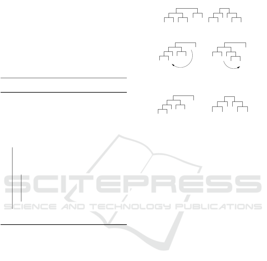
We have implemented a bottom-up iterative so-

lution (V

azquez-Ortiz et al., 2014) which compares

the subtrees present in the source and guiding solu-

tions (see Figure 2). For this the subtrees of each so-

lution are ordered by their number of leaves and we

start to compare subtrees of size 2, then subtrees of

size 3, and so on (see Algorithm 2).

Algorithm 2: Path-Relinking with bottom-up itera-

tive implementation.

input: s: source tree, g : guiding tree

output: number of transformations

1 reorder(s) ;

2 reorder(g) ;

3 trans f ormations ← 0;

4 Ω

← ordered set of subtrees of guiding tree g;

5 change ← true;

6 while change do

7 Ω

← ordered set of subtrees of source tree

8 change ← f alse ;

9 if ∃ t = (X,Y) ∈ Ω

− Ω

then

10 change ← true ;

11 degraph Y and regraph on X in s;

12 trans f ormations ←

trans f ormations + 1;

13 end

14 end

15 return trans f ormations

Consider the example of Figure 2 (a) where we

can see the source and guiding trees. First the algo-

rithm starts with subtrees of size 2 in (b) it inserts the

leave B on the node (A, F), then it transforms the node

(C,E) into the node (E,F). In the same way it con-

tinues with the subtrees of size 3 in (d) and (e).

4.1 Complexity

The complexity of the algorithm can be computed as

follows: given n, the number of taxa of the problem,

the reordering of the guiding tree needs 2n − 1 com-

parisons and the computation of Ω

can be done in

2n − 1 operations. The main loop will be executed a

certain number of times, let’s say p times, and we will

need to compute Ω

, ﬁnd a missing subtree (the ma-

ximum will be n comparisons) and perform a degraph

and regraph (1 transformation). This adds up to:

p × (2n − 1 + n + 1) + 3 × (2n − 1) ' 3n × (p + 2)

FA E

guiding tree

EA C

source tree

(a) Source and guiding trees.

F EC

A B

(b) First modiﬁ-

cation resulting in

(A,B) on source.

A B C

E F

sulting in (E,F).

A B

E F

(d) Modiﬁcation re-

sulting in ((A,B),C).

FA E

(e) Modiﬁcation re-

sulting in (D,(E,F)).

Figure 2: Example of Bottom-Up Path-Relinking with

source and guiding trees.

In the worst case p = n, so the worst case com-

plexity is O(n

) for the bottom-up implementation.

4.2 Results

4.2.1 Benchmark

We report results for a problem called zilla that was

originally obtained from the chloroplast gene rbcL

(Chase et al., 1993) and it contains 500 taxa of 759

DNA residues. Its best parsimony score of 16,218 was

found ﬁrst by TNT.

We compare the results of the bottom-up - iterative

implementation explained in this article - with the top-

down with minimization - recursive implementation

from the article of (Ribeiro and Vianna, 2009) - with

optimization on regraph, i.e. when a leaf is regraphed

all possible branches are tested and we keep the ﬁrst

one that minimizes the score of the tree.

4.2.2 Experiments

The experimentations were performed on

an Intel Core i5-4570 and the program

was coded in Java 1.7, it is part of a soft-

ware called Arbalet (http://www.info.univ-

angers.fr/pub/richer/ur.php?arbalet). In table 2

we report for each implementation the number of

transformations (degraph + regraph), the execution

time in seconds, the number of times the source

tree had a score inferior or equal to the guiding tree

(#Equal) and the number of times the source tree had

Strategies for Phylogenetic Reconstruction - For the Maximum Parsimony Problem

231

a score strictly inferior to the guiding tree (#Less)

during the generation of the path.

Note that the source tree has a higher score than

the guiding tree. This is not necessary for the bottom-

up method for which we can invert the trees. However

this is required by the top-down with minimization im-

plementation.

In Table 2, with the bottom-up implementation the

path between the two trees of score 16,218 (called

16,218 and 16,218

) was built with 24 transforma-

tions in 0.1 seconds. During the transformation pro-

cess the source tree had a best score (of 16,218) 13

times among the 24 transformations.

With the top-down with minimization algorithm

the construction of the path of the tree of score 21,727

into the tree of score 16,611 has needed 1528 trans-

formations and took 22.4 seconds. It also lead to the

generation of 586 trees of score under 16,611. This

means that the top-down with minimization algorithm

can sometimes help ﬁnd a tree of lower score than the

guiding tree.

5 SIMULATED ANNEALING

Simulated Annealing (SA) is a general-purpose

stochastic optimization technique that has proved to

be an effective tool for the approximation of global

optimal solutions to many NP-hard optimization pro-

blems. In this section we present an improved im-

plementation of a SA algorithm (see Algorithm 3)

where we applied the CPU implementation to eva-

luate the objective function because the GPU imple-

mentation requires static memory and our SA uses dy-

namic memory. We add the Path-Relinking algorithm

in the neighborhood function. The main difference

of our implementation with respect to SA of LVB

(Barker, 2003; Barker, 2012) occurs in the neighbor-

hood function (line 8) which has been tailored to be

more speciﬁc for the MP problem. Our SA employs

a composed neighborhood function combining stan-

dard neighborhood relations for trees with a stochastic

descent algorithm on the current solution, while LVB

randomly selects a neighbor s

∈ T of the current so-

lution s.

Based on previous experimentations (Vazquez-

Ortiz, 2011; Richer, 2013) we have extracted the main

components of the SA algorithm and we have used the

best values for each parameter in order to provide an

efﬁcient version of our algorithm:

• Initial solution: we use the neighbor joining (NJ)

algorithm

• Initial temperature: T

= 6.0

Algorithm 3: SA algorithm.

input: N : neighborhood, f : ﬁtness function,

MCL : Markov Chain length, α :

cooling scheme, T

: initial temperature,

: ﬁnal temperature

output: s

the best solution found

1 s

← GenerateInitialSolution();

2 s ← s

;

3 s

∗

← s

;

4 t ← T

;

5 while t > T

6 i ← 0;

7 while i < MCL do

8 s

← GenerateNeighbor(s,i,N );

9 ∆ f ← f (s

) − f (s);

10 generate a random u ∈ [0,1];

11 if (∆ f < 0) or (e

−∆ f /t

> u) then

12 s ← s

;

13 if f (s

) < f (s

∗

) then

14 s

∗

← s

;

15 end

16 end

17 i ← i + 1;

18 end

19 t ← αt;

20 end

21 return s

∗

• cooling schedule: we use a dynamic version of

the geometrical cooling schedule with a rehea-

ting system, where the temperature decreases by

a cooling factor of α = 0.99 at each step using

the relation t = αt. If the best-so-far solution is

not improved during 40 consecutive temperature

decrements, the current temperature t is increased

by a factor β = 1.4 using the function t = βt. In

our implementation this reheat mechanism can be

applied at most max reheat = 3 times, since it re-

presents a good trade-off between efﬁciency and

quality of solutions found.

• Stop condition: the algorithm terminates when the

current temperature t reaches T

= 0.0001

• Markov chain length MCL: for each temperature

t, the maximum number of visited neighboring so-

lutions is MCL. It depends directly on the parame-

ters n and k of the studied instance, since we have

observed that more moves are required for bigger

trees (Vazquez-Ortiz, 2011). For this experiment

we used MCL = 40 × (n + k)

• Neighborhood function: we use Subtree Pruning

and Regrafting (SPR) (Swofford et al., 1996). It

cuts a branch of the tree and reinserts the resulting

BIOINFORMATICS 2016 - 7th International Conference on Bioinformatics Models, Methods and Algorithms

232

Table 2: Results of Path-Relinking for Bottom-Up and Top-Down implementations (Times in seconds).

Bottom-Up Top-Down With Minimization

source / guiding Trans. Time #Equal #Less Trans. Time #Equal #Less

16218

/ 16218 24 0.10 13 0 74 0.85 21 0

16219 / 16218 32 0.14 2 0 343 4.08 3 0

16250 / 16218 97 0.40 3 0 1519 25.32 2 0

16401 / 16218 151 0.60 2 0 1474 25.36 2 0

16611 / 16218 186 0.75 2 0 1225 19.57 2 0

21727 / 16218 446 1.68 2 0 1241 18.70 2 0

16250 / 16219 92 0.37 2 0 1418 24.70 1 0

16401 / 16219 152 0.61 2 0 1390 23.74 1 0

16401 / 16250 162 0.63 1 0 1203 19.74 1 0

16611 / 16250 144 0.56 1 0 1233 35.78 3 0

21727 / 16250 449 1.71 1 0 1196 19.65 1 0

16611 / 16401 202 0.79 3 0 1216 47.75 2 1

21727 / 16611 455 1.84 2 0 1528 22.40 593 586

subtree elsewhere, generating a new internal node.

For each tree there exist 2(n − 3)(2n − 7) possi-

ble SPR neighbors (Allen and Steel, 2001) which

makes it a medium size neighborhood. N = SPR.

5.1 Computational Experiments

5.1.1 Benchmark Instances and Performance

Assessment

For our experiments we use 20 instances randomly

generated by (Ribeiro and Vianna, 2005), their gene-

rator takes as parameters the number of taxa, the num-

ber of characters, and the ratio of indeﬁnition, which

corresponds to the fraction of undeﬁned characters in

each taxon. Instances with larger ratios of indeﬁni-

tion are harder. The number of taxa in these instances

ranges from 45 to 75, the number of characters from

61 to 159, and the ratio of indeﬁnition from 20% to

50%. In the Table 3 we can see their characteristics,

in the columns two and three n represents the num-

ber of sequences and k their length, in the two last

columns we show the percentage of indeﬁnition and

similarity.

The criteria used for evaluating the performance

of the algorithms are the same as those used in the

literature: the best parsimony score found for each

instance (smaller values are better) and the expended

CPU time in seconds.

5.2 Comparison of our SA with the

State-of-the-Art Procedures

In this experiment a performance comparison of the

best solutions achieved by our SA with respect to

those produced by LVB (Barker, 2012) GA+PR+LS

Table 3: Characteristics of the instances.

Instance n k Indeﬁnition (%) Similarity (%)

tst01 45 61 20 67

tst02 47 151 30 76

tst03 49 111 40 82

tst04 50 97 50 88

tst05 52 75 20 68

tst06 54 65 30 75

tst07 56 143 40 82

tst08 57 119 50 87

tst09 59 93 20 68

tst10 60 71 30 75

tst11 62 63 40 82

tst12 64 147 50 87

tst13 65 113 20 69

tst14 67 99 30 76

tst15 69 77 40 82

tst16 70 69 50 88

tst17 71 159 20 68

tst18

73 117 30 76

tst19 74 95 40 82

tst20 75 79 50 87

(Ribeiro and Vianna, 2009), TNT (Goloboff et al.,

2008) and Hydra (Go

effon, 2006) was carried out

over the test-suite described in section 5.1.1.

The results from this experiment are depicted in

Table 4. Column 1 indicates the instance, the best

solutions found by LVB and its average CPU time are

in the second column, GA+PR+LS, TNT and Hydra,

in terms of parsimony score Φ are listed in the next

three columns. Note that for TNT this corresponds to

the best result over 30 runs. Columns 6 to 9 present

the best (B), average (Avg.), and standard deviation

(Dev.) of the parsimony score attained by our SA in

30 independent executions, as well as its average CPU

time in seconds. Finally, the difference (δ) between

the best result produced by our our SA algorithm and

the best-known solution produced by either TNT or

Strategies for Phylogenetic Reconstruction - For the Maximum Parsimony Problem

233

Table 4: Performance comparison among our SA, LVB, GA+PR+LS, TNT and Hydra over 20 standard benchmark instances.

LVB our SA

Instance Score T GA+PR+LS TNT Hydra B Avg. Dev. T δ

tst01 551 39.20 547 545 545 545 545.13 0.43 1407.57 0

tst02 1370 10.90 1361 1354 1354 1354 1355.30 0.97 1938.23 0

tst03 846 74.80 837 834 833 833 833.43 0.56 2506.30 0

tst04 595 1047.10 590 589 588 587 588.23 0.80 1341.17 -1

tst05 798 26.60 792 789 789 789 789.00 0.00 2007.90 0

tst06 605 189.80 603 597 596 596 596.57 0.56 1164.27 0

tst07 1281 84.50 1274 1273 1269 1269 1270.83 1.63 4063.80 0

tst08 875 2648.70 862 856 852 852 853.33 1.27 2884.73 0

tst09 1152 47.30 1150 1145 1144 1141 1144.73 1.09 3237.53 -3

tst10 732 408.90 722 720 721 720 720.80 0.70 2288.00 -1

tst11 551 3578.70 547 543 542 541 542.21 0.72 3807.79 -1

tst12 1234 593.70 1225 1219 1211 1208 1215.27 2.76 3668.40 -3

tst13 1533 41.60 1524 1516 1515 1515 1517.77 1.91 2514.20 0

tst14 1175 454.10 1171 1162 1160 1160 1163.03 1.82 2847.13 0

tst15 764 12427.40 758 755 752 752 753.90 1.11 4808.63 0

tst16 560 64487.00 537 531 529 529 531.00 1.23 3268.20 0

tst17 2464 40.60 2469 2453 2453 2450 2456.00 2.63 8020.23 -3

tst18 1543 179.90 1531 1522 1522 1521 1525.67 3.96 4451.37 -1

tst19 1036 3081.10 1024 1017 1013 1012 1016.23 2.14 6875.30 -1

tst20 687 56240.00 671 666 661 659 662.82 1.44 7149.43 -2

Avg. 1017.60 7285.90 1009.75 1004.30 1002.45 1001.65 1004.06 1.39 3512.51

Hydra is shown in the last column.

The analysis of the information presented in Table

4 lead us to the next observations: First, LVB (Barker,

2012) and GA+PR+LS (Ribeiro and Vianna, 2009)

return worse solutions than Hydra, TNT and our SA.

Second, the solutions provided by the proposed SA

algorithm improve all the solutions of LVB (pre-

vious SA implementation). On average our SA pro-

vided solutions with parsimony score smaller (com-

pare Columns 6 and 7) and it attained improve the

results produced by Hydra (Go

effon, 2006) on 9 best-

known solutions and to reach its results for the 11 re-

maining instances. TNT is the fastest software and

will solve a problem in a few seconds. We have no-

ticed that LVB has a erratic behavior. For example,

the resolution of problem tst15 can take from 3 min

to 14 hours and the time spent for the resolution is not

in accordance with the discovery of a better solution:

3 min to reach a solution of score 779 and 3 hours to

reach a solution of score 780.

Thus, as this experiment conﬁrms, our SA al-

gorithm is an effective alternative for solving the

MP problem, compared with the three representative

state-of-art algorithms: GA+PR+LS, TNT and Hydra.

6 CONCLUSIONS

In this paper we have described three techniques to

help improve phylogenetic reconstruction with MP:

the ﬁrst one is related to the implementation and the

evaluation of the score of a tree, the second is a stra-

tegy that could help get solutions of better quality or

could be used to compare trees. The third technique is

an adaptation of the Simulated Annealing metaheuris-

tic tailored to MP that efﬁciently could integrate the

two other strategies. From the experimentations of

this three implementations we could conclude sepa-

rately:

• CPU and GPU implementations: we have pre-

sented the implementation details of the evalua-

tion of the parsimony score of a tree on a CPU and

a GPU. The results obtained show that for a small

number of sequences of short length the CPU is

faster than the GPU. But for an important number

of sequences with a long length the GPU becomes

much faster than the CPU. This will be very in-

teresting for phylogenies based on multi-genes or

whole genomes where sequences can have from

thousands to millions of residues.

• Path-Relinking: we have described an implemen-

tation of PR in the context of Phylogenetic Recon-

BIOINFORMATICS 2016 - 7th International Conference on Bioinformatics Models, Methods and Algorithms

234

struction with Maximum Parsimony. Confronted

to other existing implementations our method

does not allow to ﬁnd trees with a better score

which is the aim of Path-Relinking but represents

an interesting tool to compare the topologies of

the source and guiding trees. The bottom-up ite-

rative implementation that we have described is

faster than the top-down recursive implementa-

tions and can serve as a measure of distance be-

tween trees and could be applied to any other con-

text.

• Simulated annealing: we have presented an im-

proved Simulated Annealing algorithm to ﬁnd

near-optimal solutions for the MP problem un-

der the optimality criterion of Fitch. In the

experiments our algorithm was carefully com-

pared with an existing Simulated Annealing

implementation (LVB) (Barker, 2003; Barker,

2012), and other three state-of-the-art algorithms

GA+PR+LS, TNT and Hydra. The results show

that our SA is able to consistently improve the

best results produced by LVB, obtaining in cer-

tain instances important reductions in the parsi-

mony score. Compared with the state-of-the-art

algorithm called Hydra (Go

effon, 2006) our SA

algorithm was able to improve on 9 previous best-

known solutions and to equal these results on the

other 11 selected benchmark instances. Further-

more, it was observed that the solution cost found

by our SA presents a relatively small standard de-

viation, which indicates the precision and robust-

ness of the proposed approach.

As future work we suggest to integrate the CUDA

evaluation technique into our implementation of Sim-

ulated Annealing for MP an use the Path-Relinking

technique to determine local optima during the de-

crease of the temperature in order to avoid unsuccess-

ful evaluations of many trees.

7 AVAILABILITY

The C++ source code for the SA algorithm and Path-

Relinking can be found on sourceforge.net under the

biosbl project. The code for the GPU implementation

is freely available from the website of Jean-Michel

Richer. It should run under all Unix/Linux platforms

(http://www.info.univ-angers.fr/pub/richer/rec.php).

REFERENCES

Allen, B. J. and Steel, M. (2001). Subtree transfer opera-

tions and their induced metrics on evolutionary trees.

Annals of Combinatorics, 5(1):1–15.

Bader, D. A., Chandu, V. P., and Yan, M. (2006). Exactmp:

An efﬁcient parallel exact solver for phylogenetic tree

reconstruction using maximum parsimony. In Parallel

Processing, 2006. ICPP 2006. International Confer-

ence on, pages 65–73. IEEE.

Barker, D. (2003). LVB: parsimony and simulated annea-

ling in the search for phylogenetic trees. Bioinformat-

ics, 20(2):274–275.

Barker, D. (2012). LVB homepage.

Chase, M. W., Soltis, D. E., Olmstead, R. G., Morgan,

D., Les, D. H., Mishler, B. D., Duvall, M. R., Price,

R. A., Hills, H. G., Qiu, Y., Kron, K. A., Rettig,

J. H., Conti, E., Palmer, J. D., Manhart, J. R., Sytsma,

K. J., Michaels, H. J., Kress, W. J., Karol, K. G.,

Clark, W. D., Hedren, M., Gaut, B. S., Jansen, R. K.,

Kim, K., Wimpee, C. F., Smith, J. F., Furnier, G. R.,

Strauss, S. H., Xiang, Q., Plunkett, G. M., Soltis, P. S.,

Swensen, S. M., Williams, S. E., Gadek, P. A., Quinn,

C. J., Eguiarte, L. E., Golenberg, E., Learn, G. H.,

Graham, S. W., Barrett, S. C. H., Dayanandan, S., and

Albert, V. A. (1993). Phylogenetics of seed plants:

An analysis of nucleotide sequences from the plastid

gene rbcl. Annals of the Missouri Botanical Garden,

80(3):528–580.

Felsenstein, J. (2003). Inferring phylogenies. Sinauer As-

sociates.

Fitch, W. (1971). Towards deﬁning course of evolution:

minimum change for a speciﬁed tree topology. Sys-

tematic Zoology, 20:406–416.

Foulds, L. R. and Graham, R. L. (1982). The steiner pro-

blem in phylogeny is np-complete. Advances in Ap-

plied Mathematics, 3(1):43–49.

Gladstein, D. S. (1997). Efﬁcient incremental character op-

timization. Cladistics, 13(1-2):21–26.

Glover, F., Laguna, M., and Mart, R. (2000). Fundamen-

tals of scatter search and path relinking. Control and

Cybernetics, 39:653–684.

effon, A. (2006). Nouvelles heuristiques de voisinage

et m

etiques pour le probl

eme maximum de parci-

monie. PhD thesis, LERIA, Universit

e d’Angers.

Goloboff, P. (1999). Analyzing large data sets in reason-

able times: solutions for composite optima. Cladis-

tics, 15:415–428.

Goloboff, P. (2002). Techniques for analyzing large data

sets. In DeSalle R., G. G. and Wheeler W., e., editors,

Techniques in Molecular Systematics and Evolution,

page 7079. Brikhuser Verlag, Basel.

Goloboff, P. A. (1993). Nona, version 2.0. Computer Pro-

gram and Manual Distributed by the Author.

Goloboff, P. A., Farris, J. S., and Nixon, K. C. (2008). Tnt,

a free program for phylogenetic analysis. Cladistics,

24(5):774–786.

Gusﬁeld, D. (1997). Algorithms on strings, trees, and se-

quences: Computer science and computational biol-

ogy. Cambridge University Press, 1st. edition.

Hartigan, J. A. (1973). Minimum mutation ﬁts to a given

tree. Biometrics, 29:53–65.

Strategies for Phylogenetic Reconstruction - For the Maximum Parsimony Problem

235

Hendy, M. D. and Penny, D. (1982). Branch and bound

algorithms to determine minimal evolutionary trees.

Mathematical Biosciences, 59(2):277–290.

Hennig, W. (1966). Phylogenetic systematics. Phylogeny.

University of Illinois Press, Urbana.

Hillis, D. M., Moritz, C., and Mable, B. K. (1996). Molecu-

lar systematics. Sinauer Associates Inc., Sunderland,

MA, 2nd. edition.

Kasap, S. and Benkrid, K. (2011). High performance phy-

logenetic analysis with maximum parsimony on re-

conﬁgurable hardware. Very Large Scale Integration

(VLSI) Systems, IEEE Transactions on, 19(5):796–

808.

Maddison, D. R. (1991). The discovery and importance of

multiple islands of most-parsimonious trees. System-

atic Zoology, 40(3):315–328.

Penny, D., Foulds, L. R., and Hendy, M. D. (1982). Test-

ing the theory of evolution by comparing phyloge-

netic trees constructed from ﬁve different protein se-

quences. Nature, 297:197–200.

Ribeiro, C. C. and Vianna, D. S. (2005). A GRASP/VND

heuristic for the phylogeny problem using a new

neighborhood structure. International Transactions in

Operational Research, 12(3):325–338.

Ribeiro, C. C. and Vianna, D. S. (2009). A hybrid ge-

netic algorithm for the phylogeny problem using path-

relinking as a progressive crossover strategy. In-

ternational Transactions in Operational Research,

16(5):641–657.

Richer, J.-M. (2008). Three new techniques to im-

prove phylogenetic reconstruction with maximum

parsimony. Technical report, LERIA, University of

Angers, France.

Richer, J.-M. (2013). Improvevement of ﬁtch function for

maximum parsimony in phylogenetic reconstruction

with intel avx2 assembler instructions. Technical re-

port, LERIA, University of Angers, France.

Richer, J. M., Go

effon, A., and Hao, J. K. (2009). A

memetic algorithm for phylogenetic reconstruction

with maximum parsimony. Lecture Notes in Computer

Science, 5483:164–175.

Ronquist, F. (1998a). Fast ﬁtch-parsimony algorithms for

large data sets. Cladistics, 14(4):387–400.

Ronquist, F. (1998b). Fast ﬁtch-parsimony algorithms for

large data sets. Cladistics, 14(4):387–400.

Sober, E. (1993). The nature of selection: Evolutionary

theory in philosophical focus. University Of Chicago

Press.

Sridhar, S., Lam, F., Blelloch, G. E., Ravi, R., and Schwartz,

R. (2007). Direct maximum parsimony phylogeny re-

construction from genotype data. BMC Bioinformat-

ics, 8(472).

Swofford, D. L., Olsen, G. J., Waddell, P. J., and Hillis,

D. M. (1996). Phylogeny reconstruction. In Molec-

ular Systematics, chapter 11, pages 411–501. Sinauer

Associates, Inc., Sunderland, MA, 2nd. edition.

Vazquez-Ortiz, K. E. (2011). Metaheur

ısticas para la res-

oluci

on del problema de m

axima parsimonia. Mas-

ter’s thesis, LTI, Cinvestav - Tamaulipas, Cd. Vitoria,

Tamps. Mexico.

azquez-Ortiz, K. E., Richer, J.-M., Lesaint, D., and

Rodriguez-Tello, E. (2014). A bottom-up implemen-

tation of path-relinking for phylogenetic reconstruc-

tion applied to maximum parsimony. In Computa-

tional Intelligence in Multi-Criteria Decision-Making

(MCDM), 2014 IEEE Symposium on, pages 157–163.

IEEE.

White, W. T. J. and Holland, B. R. (2011). Faster exact ma-

ximum parsimony search with xmp. Bioinformatics,

27(10):1359–1367.

Xiong, J. (2006). Essential Bioinformatics. Cambridge Uni-

versity Press, 1st. edition.

BIOINFORMATICS 2016 - 7th International Conference on Bioinformatics Models, Methods and Algorithms

236