Sparse Physics-based Gaussian Process for Multi-output Regression

using Variational Inference

Ankit Chiplunkar

1,3

, Emmanuel Rachelson

, Michele Colombo

and Joseph Morlier

Airbus Operations S.A.S., 316 route de Bayonne 31060, Toulouse Cedex 09, France

Universit

e de Toulouse, ISAE, DISC, 10 Avenue Edouard Belin, 31055 Toulouse Cedex 4, France

Universit

e de Toulouse, CNRS, ISAE-SUPAERO, Institut Cl

ement Ader (ICA), 31077 Toulouse Cedex 4, France

Keywords:

Gaussian Process, Kernel Methods, Variational Inference, Multi-output Regression, Flight-test data.

Abstract:

In this paper a sparse approximation of inference for multi-output Gaussian Process models based on a Vari-

ational Inference approach is presented. In Gaussian Processes a multi-output kernel is a covariance function

over correlated outputs. Using a general framework for constructing auto- and cross-covariance functions that

are consistent with the physical laws, physical relationships among several outputs can be imposed. One major

issue with Gaussian Processes is efﬁcient inference, when scaling up-to large datasets. The issue of scaling

becomes even more important when dealing with multiple outputs, since the cost of inference increases rapidly

with the number of outputs. In this paper we combine the use of variational inference for efﬁcient inference

with multi-output kernels enforcing relationships between outputs. Results of the proposed methodology for

synthetic data and real world applications are presented. The main contribution of this paper is the applica-

tion and validation of our methodology on a dataset of real aircraft ﬂight tests, while imposing knowledge of

aircraft physics into the model.

1 INTRODUCTION

In this work we consider the problem of modelling

multiple output Gaussian Process (GP) regression

(Rasmussen and Williams, 2005) correlated through

physical laws of the system, while in presence of

large number of inputs. In the literature inference

on multiple output data is also known as co-kriging

(Stein, 1999) or multi-kriging (Boyle and Frean,

2005). Modelling multi-output kernels is particularly

difﬁcult because we need to construct auto- and cross-

covariance functions between different outputs. We

turn to a general framework (Constantinescu and An-

itescu, 2013) to calculate these covariance functions

while imposing prior information of the physical pro-

cesses. While a joint model developed using corre-

lated covariance functions gives better predictions, it

incurs a huge cost on memory occupied and computa-

tional time. The main contribution of this paper is to

apply variational inference on these models of large

datasets (of the order O(10

))and reduce the heavy

computational costs incurred.

Let us start by deﬁning a P dimensional input

space and a D dimensional output space. Such that

{(x

, y

)} for j ∈ [1;n

] are the training datasets for

the i

output. Here n

is the number of measure-

ment points for the i

output, while x

∈ R

and

∈ R. We next deﬁne x

= {x

;. . . ;x

} and y

;. . . ;y

} as the full matrices containing all the

training points for the i

output such that x

∈ R

×P

and y

∈ R

. Henceforth we deﬁne the joint output

vector Y = [y

;. . . ;y

] such that all the output

values are stacked one after the other. Similarly, we

deﬁne the joint input matrix as X = [x

, x

, . . . , x

If Σn

= N for i ∈ [1, D]. Hence N represents the to-

tal number of training points for all the outputs com-

bined. Then Y ∈ R

and X ∈ R

N×P

For simplicity take the case of an explicit relation-

ship between two outputs y

and y

. Suppose we mea-

sure two outputs with some error, while the true phys-

ical process is deﬁned by latent variables f

and f

Then the relation between the output function, mea-

surement error and true physical process can be writ-

ten as follows.

= f

+ ε

= f

+ ε

(1)

Where, ε

and ε

are measurement error sam-

pled from a white noise gaussian N (0, σ

) and

Chiplunkar, A., Rachelson, E., Colombo, M. and Morlier, J.

Sparse Physics-based Gaussian Process for Multi-output Regression using Variational Inference.

DOI: 10.5220/0005700504370445

In Proceedings of the 5th International Conference on Pattern Recognition Applications and Methods (ICPRAM 2016), pages 437-445

ISBN: 978-989-758-173-1

437

N (0, σ

). While the physics based relation can be

expressed as,

= g ( f

, x

) (2)

Here g is an operator deﬁning the relation between

and an independent latent output f

. A GP prior in

such a setting with 2 output variables is:





∼ GP







+ σ



(3)

and K

are cross-covariances between the two

inputs x

and x

. K

is the covariance function of

independent output, σ

and σ

are the variance of

measurement error, while K

is the auto-covariance

of the dependent output variable. m

and m

are the

mean of the prior for outputs 1 and 2. The full covari-

ance matrix is also called the joint kernel, henceforth

we will denote the joint-kernel as K





(4)

while the joint error matrix will be denoted by Σ;

Σ =



0 σ



(5)

Full joint-kernel of a multi-output GP has huge

memory and computational costs. For a multi-output

GP as deﬁned earlier the covariance matrix is of

size N, needing O





calculations for inference

and O





for storage. (Snelson and Ghahramani,

2006) introduced “Fully independent training condi-

tional” (FITC) and (Quionero-candela et al., 2005) in-

troduced and “Partially Independent Training Condi-

tional” (PITC) approximations on inference of a GP

using inducing inputs. Later (Alvarez and Lawrence,

2009) extended the application of FITC and PITC to

approximate the inference of multi-output GP’s con-

structed through convolution processes. One prob-

lem with FITC and PITC approximation is their ten-

dency to over-ﬁt. In this work we extend the use

of a variational approach (Titsias, 2009) to approxi-

mate the inference in a joint-kernel for both linear and

non-linear relationships. We observe that the current

approximation reduces the computational complexity

to O



N(MD)



and storage to O (NMD), where M

denotes the number of inducing points in the input

space.

In Section 2, we start with an introduction to

multi-output GP and later derive the multi-output GP

regression in presence of correlated covariances. In

Section 3 we discuss various methods of approximat-

ing inference of a GP and later derive application of

variational inference on the problem of multi-output

kernels. Finally, in Section 4 we demonstrate the ap-

proach on both theoretical and ﬂight-test data.

2 MULTI-OUTPUT GAUSSIAN

PROCESS

Choosing covariance kernels for GP regression with

multiple outputs can be roughly classiﬁed in three cat-

egories. In the ﬁrst case, the outputs are known to be

mutually independent, and thus the system can be de-

coupled and solved separately as two or more unre-

lated problems. In the second case, we assume that

the processes are correlated, but we have no infor-

mation about the correlation function. In this case, a

model can be proposed, or nonparametric inferences

can be carried out. In the third situation, we assume

that the outputs have a known relationship among

them, such as equation 2. The last point forms the

scope of this section.

2.1 Related Work

Earlier work developing such joint covariance func-

tions (Bonilla et al., 2008) have focused on build-

ing different outputs as a combination of a set of la-

tent functions. GP priors are placed independently

over all the latent functions thereby inducing a cor-

related covariance function. More recently (Alvarez

et al., 2009) have shown how convolution processes

(Boyle and Frean, 2005) can be used to develop

joint-covariance functions for differential equations.

In a convolution process framework output functions

are generated by convolving several latent functions

with a smoothing kernel function. In the current

paper we assume one output function to be inde-

pendent and evaluate the remaining auto- and cross-

covariance functions exactly if the physical relation

between them is linear (Solak et al., 2003) or use

approximate joint-covariance for non-linear physics-

based relationships between the outputs (Constanti-

nescu and Anitescu, 2013).

2.2 Multi-output Joint-covariance

Kernels

If the two outputs y

and y

satisfy a physical relation-

ship given by equation 2 with g (.) ∈ C

, and known

covariance matrix K

. Then the joint-covariance ma-

trix for a linear operator g(.) can be derived analyti-

cally as (Stein, 1999):



g(g(K

, x

), x

) g(K

, x

)

g(K

, x

) K



(6)

Since a non-linear operation on a GP does not re-

sult in a GP, for the case of non-linear g (.) the above

joint-covariance matrix as derived in equation 6 is not

ICPRAM 2016 - International Conference on Pattern Recognition Applications and Methods

438

positive semi-deﬁnite. Therefore we will use an ap-

proximate joint-covariance as developed by (Constan-

tinescu and Anitescu, 2013) for imposing non-linear

relations:





+ O



δy



(7)

Where L =

∂g

∂y



= ¯y

is the Jacobian matrix of g (.)

evaluated at the mean of independent output y

. δy

the amplitude of small variations of y

, introduced by

the Taylor series expansion of g(K

) with respect to

The above kernel takes a parametric form that de-

pends on the mean value process of the independent

variable. Equation 7 is basically a Taylor series ex-

pansion for approximating related kernels. Since a

Taylor series expansion is constructed from deriva-

tives of a function which are linear operations the re-

sulting approximated joint kernel is a gaussian kernel

with the non-gaussian part as the error. Higher-order

closures can be derived with higher order derivatives

of the relation g(.). For simplicity we will restrict

ourselves to ﬁrst order approximation of the auto- and

cross-covariance functions leading to an error of the

order O



δy



. (Constantinescu and Anitescu, 2013)

provide a more detailed derivation of equation 7.

2.3 GP Regression using

Joint-covariance

We start with deﬁning a zero-mean prior for our ob-

servations and make predictions for y

∗

) = y

∗1

and

∗

) = y

∗2

. The corresponding prior according to

equation 3 and 4 will be:



Y (X))

Y (X

∗

))



= GP







+ Σ K

∗

+ Σ



(8)

The predictive distribution is then given as a nor-

mal distribution with expectation and covariance ma-

trix given by (Rasmussen and Williams, 2005)

∗

| X , X

∗

, Y = K

∗

)

−1

Y (9)

Cov (Y

∗

| X, X

∗

, Y ) = K

∗

− K

∗

)

−1

∗

(10)

Here, the elements K

, K

∗

and K

∗

are block

covariances derived from equations 6 or 7.

The joint-covariance matrix depends on several

hyperparameters θ. They deﬁne a basic shape of the

GP prior. To end up with good predictions it is impor-

tant to start with a good GP prior. We minimize the

negative log-marginal likelihood to ﬁnd a set of good

hyperparameters. This leads to an optimization prob-

lem where the objective function is given by equation

log(P(y | X, θ)) = log[GP(Y |0, K

+ Σ)] (11)

With its gradient given by equation 12

∂

∂θ

log(P(y | X, θ)) =

−1

∂K

∂θ

−1

−

tr(K

−1

∂K

∂θ

) (12)

Here the hyperparameters of the prior are θ =



, σ



. These correspond to the hyperpa-

rameters of the independent covariance function K

and errors in the measurements σ

and σ

. Calculat-

ing the negative log-marginal likelihood involves in-

verting the matrix K

+ Σ. The size of the K

+ Σ

matrix depends on total number of input points N,

hence inverting the matrix becomes intractable for

large number of input points.

In the next section we describe how to solve the

problem of inverting huge K

+ Σ matrices using

sparse GP regression. We also elaborate on how varia-

tional approximation overcomes the problem of over-

ﬁtting by providing a distance measure between two

approximate models.

3 SPARSE GP REGRESSION

The above GP approach is intractable for large

datasets. For a multi-output GP as deﬁned in sec-

tion 2.2 the covariance matrix is of size N, where





time is needed for inference and O





mem-

ory for storage. Thus, we need to consider approx-

imate methods in order to deal with large datasets.

Sparse methods use a small set of m function points

as support or inducing variables.

Suppose we use m inducing variables to construct

our sparse GP. The inducing variables are the latent

function values evaluated at inputs x

. Learning x

and the hyperparameters θ is the problem we need

to solve in order to obtain a sparse GP method. An

approximation to the true log marginal likelihood in

equation 11 can allow us to infer these quantities.

3.1 Related Work

Before explaining variational inference method, we

review FITC method proposed by (Snelson and

Ghahramani, 2006). The approximate log-marginal

likelihoods have the form

F = log[GP(y|0, Q

+ Σ)] (13)

Sparse Physics-based Gaussian Process for Multi-output Regression using Variational Inference

439

where Q

is an approximation to the true covariance

. In FITC approach, the Q

takes the form,

= diag[K

− K

−1

] + K

−1

(14)

Here, K

is a m × m covariance matrix on inducing

points x

, K

is a n × m cross-covariance matrix be-

tween the training and inducing points.

Hence the position of x

now deﬁnes the approx-

imated marginal likelihood. The maximization of the

marginal likelihood in equation 13 with respect to

; θ), is prone to over-ﬁtting especially when the

number of variables in x

is large. Fitting a modi-

ﬁed sparse GP model implies that the full GP model

is not approximated in a systematic way since there is

no distance measure between the two models that is

minimized.

3.2 Variational Approximation

During variational approximation, we seek to apply

an approximate variational inference procedure where

we introduce a variational distribution q(x) to approx-

imate the true posterior distribution p(x|y). We take

the variational distribution to have a factorized Gaus-

sian form as given in equation 15

q(x) = N (x|µ, A) (15)

Here, µ and A are parameters of the variational distri-

bution. Using this variational distribution we can ex-

press a Jensens lower bound on the logP(y) that takes

the form:

F(q) =

q(x)log

p(y|x)p(x)

q(x)

q(x)logp(y|x)dx −

q(x)log

q(x)

p(x)

− KL(q||p) (16)

Where the second term is the negative Kullback

Leibler divergence between the variational posterior

distribution q(x) and the prior distribution p(x). To

determine the variational quantities (x

, θ), we mini-

mize the KL divergence KL(q||p). This minimization

is equivalently expressed as the maximization of the

variational lower bound of the true log marginal like-

lihood

= log(N [y|0, σ

I + Q

]) −

2σ

Tr(

K) (17)

where Q

= K

−1

and

K = K

−

−1

. The novelty of the above objec-

tive function is that it contains a regularization

trace term: −

2σ

Tr(

K). Thus, F

attempts to

maximize the log likelihood Q

and simultaneously

minimize the trace Tr(

K). Tr(

K) represents the

total variance of the conditional prior. When Tr(

= 0, K

= K

−1

, which means that the

inducing variables can exactly reproduce the full GP

prediction.

3.3 Variational Approximation on

Multi-output GP

(

Alvarez et al., 2010) derived a variational approxi-

mation to inference of multi-output regression using

convolution processes. They introduce the concept of

variational inducing kernels that allows them to efﬁ-

ciently sparsify multi-output GP models having white

noise latent functions. White noise latent functions

are needed while modelling partial differential equa-

tions. These variational inducing kernels are later

used to parametrize the variational posterior q(X).

For our expression of the joint kernel, the auto-

and cross-covariance functions are dependent on the

independent covariance function K

. Hence the in-

dependent output function in our case behaves like a

latent function for the case of (

Alvarez et al., 2010).

Moreover, the latent function or independent output

is a physical process and hence will almost never be

white noise. Henceforth we will place the inducing

points on the input space. We now extend the varia-

tional inference method to deal with multiple outputs.

We try to approximate the joint-posterior distribu-

tion p(X|Y ) by introducing a variational distribution

q(X). In the case of varying number of inputs for

different outputs, we place the inducing points over

the input space and extend the derivation of (Titsias,

2009) to multi-output case.

q(X) = N (X|µ, A) (18)

Here µ and A are parameters of the variational dis-

tribution. We follow the derivation provided in sec-

tion 3.2 and obtain the lower bound of true marginal

likelihood.

= log(N [Y |0, σ

I + Q

]) −

2σ

Tr(

K) (19)

where Q

= K

−1

and

K = K

−

−1

. K

is the joint-covariance matrix

derived using equation 6 or 7 using the input vector

X deﬁned in section 1. K

is the joint covari-

ance function on the inducing points X

, such that

= [x

, x

, ..., x

]. We assume that the induc-

ing points x

will be same for all the outputs, hence

ICPRAM 2016 - International Conference on Pattern Recognition Applications and Methods

440

= x

= ... = x

= x

. While K

is the cross-

covariance matrix between X and X

Note that this bound consists of two parts. The

ﬁrst part is the log of a GP prior with the only differ-

ence that now the covariance matrix has a lower rank

of MD. This form allows the inversion of the covari-

ance matrix to take place in O



N(MD)



time. The

second part as discussed above can be seen as a pe-

nalization term that regularizes the estimation of the

parameters.

The bound can be maximized with respect to all

parameters of the covariance function; both model hy-

perparameters and variational parameters. The opti-

mization parameters are the inducing inputs x

, the

hyperparameters θ of the independent covariance ma-

trix K

and the error while measuring the outputs

Σ. There is a trade-off between quality of the es-

timate and amount of time taken for the estimation

process. On the one hand the number of inducing

points determine the value of optimized negative log-

marginal likelihood and hence the quality of the es-

timate. While, on the other hand there is a computa-

tional load of O



N(MD)



for inference. We increase

the number of inducing points until the difference be-

tween two successive likelihoods is below a prede-

ﬁned quantity.

4 NUMERICAL RESULTS

In this section we provide numerical illustration to

the theoretical derivations in the earlier sections. We

start with a synthetic problem where we try to learn

the model over derivative and quadratic relationships.

We compare the error values for the variational ap-

proximation with respect to the full GP approach. Fi-

nally we look at the results in presence of a real world

dataset related to ﬂight loads estimation.

The basic toolbox used for this paper is GPML

provided with (Rasmussen and Williams, 2005), we

generate covariance functions to handle relationships

as described in equations 6 and 7 using the ”Sym-

bolic Math Toolbox” in MATLAB 2014b. Since vari-

ational approximation was not coded in GPML we

have wrapped the variational inference provided in

gpStuff (Vanhatalo et al., 2013) in the GPML tool-

box. All experiments were performed on an Intel

quad-core processor with 4Gb RAM.

4.1 Numerical Results on Theoretical

Data

We begin by considering the relationship between two

latent output functions as described in equation 2.

Such that

∼ GP[0, K

(0.1, 1)]

∼ N [0, 0.2]

∼ N [0, 2] (20)

(0.1, 1) means squared exponential kernel

with length scale 0.1 and variance as 1.

4.1.1 Differential Relationship

We take the case of a differential relationship g(.),

such that g( f , x) =

∂ f

∂x

. Since the differential relation-

ship g(.) is linear in nature we use the equation 6 to

calculate the auto- and cross-covariance functions as

shown in table 1.

Table 1: Auto- and cross-covariance functions for a differ-

ential relationship.

Initial Covariance K

exp(

−1

)

Cross-Covariance K

exp(

−1

)

Auto-covariance K

−l

exp(

−1

)

To generate data a single function is drawn from

as described in equation 20 which then is used to

calculate y

and y

. 10,000 training points are gener-

ated for both the outputs. Values of y

for x ∈ [0, 0.3]

are removed from the training points. Next we opti-

mize the lower bound of log-marginal likelihood us-

ing variational inference, for independent GP’s on y

and y

as described in 3.2. Later we optimize the same

lower bound but with a joint-covariance approach as

described in section 3.3 using y

, y

and g(.). As

explained in section 3.3 we settled on using 100 in-

ducing points for this experiment because there was

negligible increase in lower bound F

of log-marginal

likelihood upon increasing the inducing points.

In ﬁgure 1(a) we show the independent (blue

shade) and joint ﬁt (red shade) of two GP for the dif-

ferential relationship. The GP model with joint co-

variance gives better prediction even in absence of

data of y

for x ∈ [0, 0.3] because transfer of infor-

mation is happening from observations of y

present

at those locations. Nonetheless we see an increase

in variance at masked ’x’ values even for joint-

covariance kernel. The distribution of inducing points

may look even in the diagram but are uneven at places

where we have removed the data from y

Sparse Physics-based Gaussian Process for Multi-output Regression using Variational Inference

441

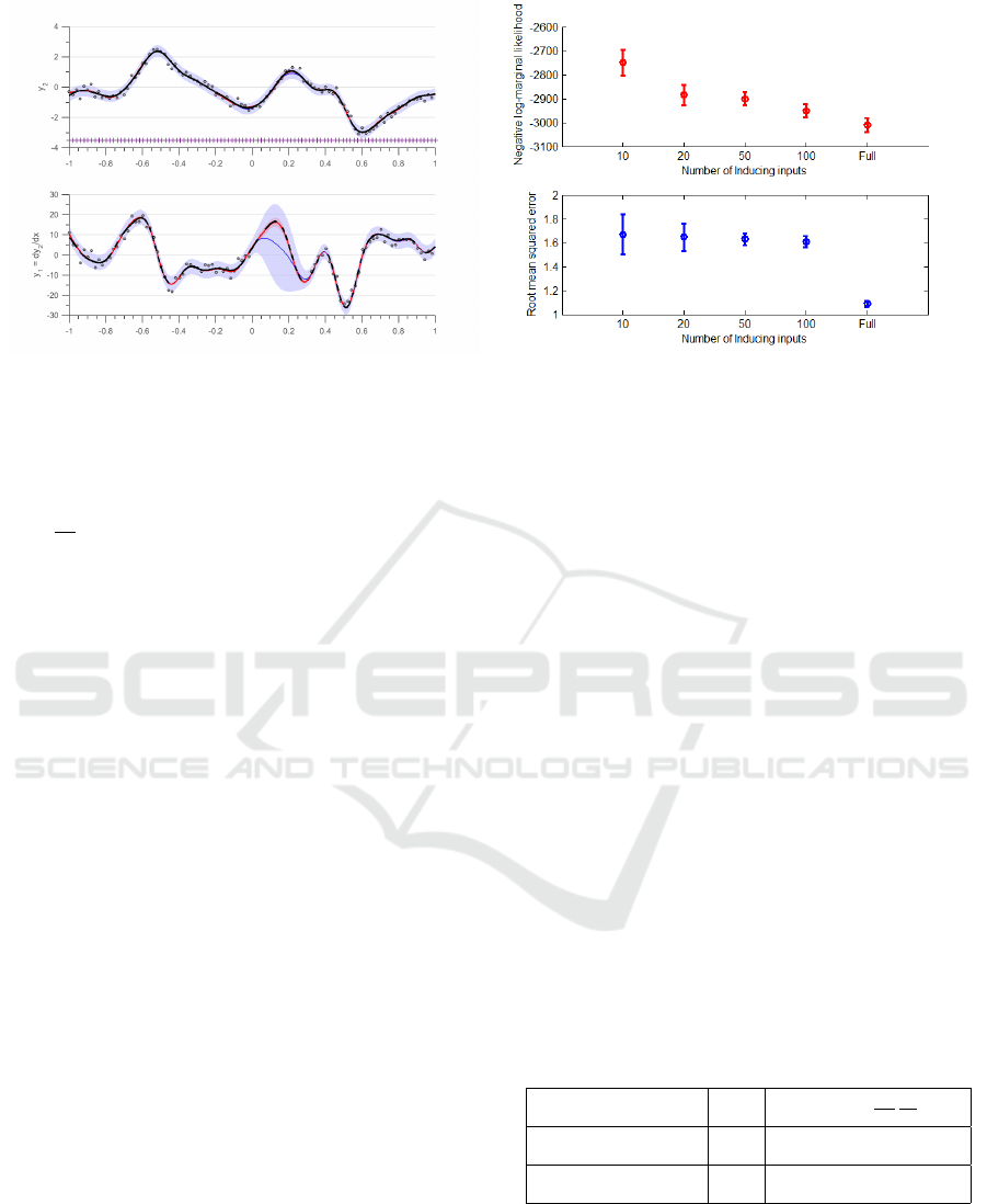
(a) Independent ﬁt for two GP’s in blue variance is repre-

sented by light blue region and mean is represented by solid

blue line. Variance and mean of the dependent are repre-

sented in red region and solid red line. The dashed black

line represents the true latent function values; noisy data is

denoted by circles. Experiment was run on 10,000 points but

only 100 data points are plotted to increase readibility.Here

∂ f

∂x

, y

= f

+ σ

and y

= f

+ σ

. The + points

refer to the location of the inducing points in the inference.

(b) The ﬁgure shows progression of different measures upon

increasing number of inducing points from 10, 20, 50 to 100

and ﬁnally full Multi-output physics based GP. The top ﬁg-

ure in red shows the value of mean and variance of nega-

tive log-marginal likelihood, while the bottom ﬁgure in blue

shows the mean and variance of root mean squared error. 10

sets of experiments were run on 75% of the data as training

set and 25% of the data as the test set, the training and test

sets were chosen randomly.

Figure 1: Experimental results for differential relationship with approximate inference using variational approximation.

For the second experiment we generate 1000

points and compare the Root Mean Squared Error

(RMSE) and log-marginal likelihood between full re-

lationship kernel as described in section 2.3 and vari-

ational inference relationship kernel as described in

section 3.3, using 10, 20, 50 and 100 inducing points.

10 sets of experiments were run on 75% of the data

as training set and 25% of the data as the test set, the

training and test sets were chosen randomly. We learn

the optimal values of hyper-parameters and inducing

points for all the 10 sets of experiments of training

data. Finally, RMSE values are evaluated with respect

to the test set and negative log-marginal likelihood are

evaluated for each learned model. The RMSE values

are calculated for only the dependent output y

and

then plotted in the ﬁgures below.

In ﬁgure 1(b) the mean and variance of negative

log-marginal likelihood for 10 sets of experiments are

calculated with varying number of inducing inputs

at the top in red. As expected upon increasing the

number of inducing points we see that the values of

mean negative log-marginal likelihood tends to be-

come an asymptote reaching the value of mean nega-

tive log-marginal likelihood of a full multi-output GP.

In the bottom ﬁgure we have the mean and variance

of RMSE for 10 sets of experiments. We see that the

mean value of RMSE does not vary drastically upon

increasing the inducing points but the value of vari-

ance gets reduced. One can observe an almost con-

stant RMSE in ﬁgure 1(b) with a sudden decrease for

a full GP (as M tends to N). Although this behaviour

was expected, providing an explanation for the slow

decrease with low values of M requires further inves-

tigation.

4.1.2 Quadratic Relationship

Now we take the case of a quadratic relationship g(.),

such that g( f , x) = f

. Since the quadratic relation-

ship g(.) is non-linear in nature we use the equation 7

to calculate the auto- and cross-covariance functions

as shown in table 2. The Jacobin L for this case be-

comes 2

(x). Here the value of

(x) is the mean

value of the latent-independent output function f

cal-

culated at the input point x.

Table 2: Auto- and cross-covariance functions for a

quadratic relationship.

Initial Covariance K

exp(

−1

)

Cross-Covariance K

(x)K

Auto-covariance K

(x)

+ 2K

)

As stated in the earlier section 4.1.1 the output

data was generated using the same draw of f

as ex-

plained in equation 20. 10,000 training points are gen-

erated for both the outputs. Values of y

for x ∈ [0, 0.3]

are removed from the training points. Note that the

above calculated auto- and cross-covariances are third

ICPRAM 2016 - International Conference on Pattern Recognition Applications and Methods

442

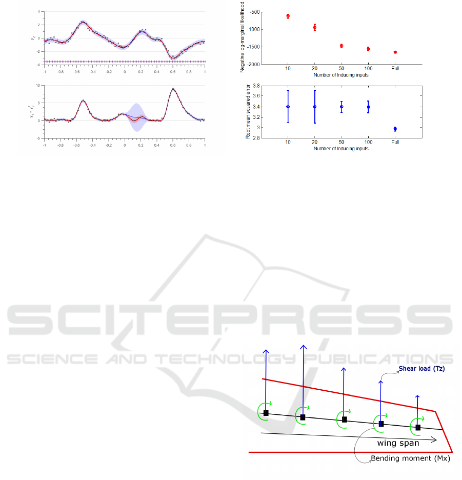
(a) Independent ﬁt for two GP in blue variance is rep-

resented by light blue region and mean is represented

by solid blue line. Variance and mean of the depen-

dent are represented in red region and solid red line.

The dashed black line represents the true latent function

values; noisy data is denoted by circles only 100 data

points are plotted to increase readibility. Here f

= f

+ σ

and y

= f

+ σ

. The + points refer to

the location of the inducing points in the inference.

(b) The ﬁgure shows progression of different measures

upon increasing number of inducing points from 10, 20,

50 to 100 and ﬁnally full Multi-output physics based GP.

The top ﬁgure in red shows the value of mean and vari-

ance of negative log-marginal likelihood, while the bot-

tom ﬁgure in blue shows the mean and variance of root

mean squared error. 10 sets of experiments were run on

75% of the data as training set and 25% of the data as the

test set, the training and test sets were chosen randomly.

Figure 2: Experimental results for quadratic relationship with approximate inference using variational approximation.

order Taylor series approximations as presented in

equation 7.

Calculating the Jacobin

(x) at the inducing and

input points was a requirement of the algorithm.

Moreover, during the optimization process the value

of x

keeps on changing, since the

) depends

on the value of x

. Many a times we don’t have

value of latent independent output function at these

new points. To solve this problem we ﬁrst learn an in-

dependent model of the output y

recover an estimate

(x) and use this value to calculate the required

auto- and cross-covariances.

In ﬁgure 2(a) we show the independent and joint

ﬁt of two GP for the quadratic relationship. Even

in the presence of the error the joint-covariance GP

model gives better prediction because of transfer of

information. The GP model with joint covariance

gives better prediction even in absence of data of y

for x ∈ [0, 0.3] because transfer of information is hap-

pening from the observations of y

present at those

locations.

Upon performing the second experiment as de-

scribed in section 4.1.1 we get the ﬁgure 2(b). The

top part in the ﬁgure is the mean and variance of neg-

ative log-marginal likelihood for varying number of

inducing points. We see that the value mean nega-

tive log-marginal likelihood reaches the value of full

negative log-marginal likelihood. In the lower ﬁgure

we have mean and variance of RMSE of the depen-

dent output y

. As seen in the earlier experiment we

observe high amount of variance for lower inducing

points due to the approximate nature.

4.2 Numerical Results on Flight Test

Data

Figure 3: Wing Load Diagram.

In this section we conduct experiments, applying our

approach on the ﬂight loads data recovered during

ﬂight test campaigns at Airbus. We look at normal-

ized data of a simple longitudinal maneuver. The two

outputs in our case are shear load T

and bending mo-

ment M

as described in ﬁgure 3. The input space is

2-dimensional space with wing span η or point of ac-

tion of forces as he ﬁrst input variable and angle of

attack α as the second input variable. The maneuver

is quasi-static which means that airplane is in equi-

librium at all time and there are no dynamic effects

observed by the aircraft. The relation between T

and

Sparse Physics-based Gaussian Process for Multi-output Regression using Variational Inference

443

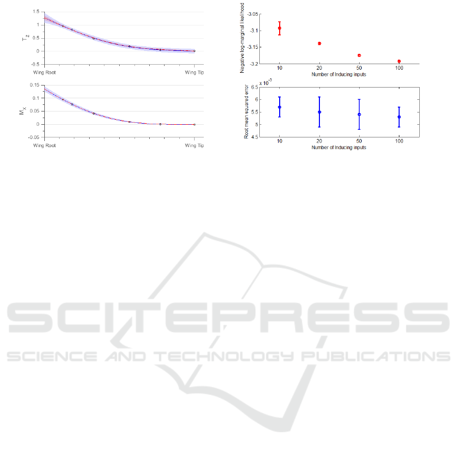
(a) Independent ﬁt for two GP in blue variance is rep-

resented by light blue region and mean is represented

by solid blue line. Variance and mean of the depen-

dent are represented in red region and solid red line. The

dashed black line represents the true latent function val-

ues; noisy data is denoted by circles only 1 α step is

plotted.

(b) The ﬁgure shows progression of different measures

upon increasing number of inducing points from 10, 20,

50 to 100. The top ﬁgure in red shows the value of mean

and variance of negative log-marginal likelihood, while

the bottom ﬁgure in blue shows the mean and variance

of root mean squared error.

Figure 4: Experimental results for aircraft ﬂight loads data with approximate inference using variational approximation.

can be written as:

(η, α) =

edge

(x, α)(x − η)dx. (21)

Note that the above equation is calculated only

on the η axis. Here, η

edge

denotes the edge of the

wing span. The above equation is linear in nature

and hence we will use equation 6 to calculate the

auto- and cross-covariance functions. The forces are

measured at 5 points on the wing span and at 8800

points in the second axis. We follow the procedure

described in earlier experiments where we compare

plots of relationship-imposed multioutput GP and in-

dependent GP. Secondly, we compare the measures of

negative-log marginal likelihood and RMSE for vary-

ing number of inducing points.

In ﬁgure 4(a) we see the plot of independent and

dependent T

at the top with the dependent plot in red

and independent plot in blue. In the bottom part of

ﬁgure we show the plot for M

. Only one α is plot-

ted here for better viewing. 100 inducing points in

the input space are used to learn and plot the ﬁgure.

We see that the region in red, has a tighter variance

than the one in blue conﬁrming the improvement by

our method. The relationship in equation 21 is acting

as extra information in tightening the error margins of

the loads estimation. This becomes very useful when

we need to identify faulty data because the relation-

ship will impose a tighter bound on the variance and

push faulty points out of the conﬁdence interval.

In ﬁgure 4(b) we see how the negative log-

marginal likelihood and RMSE plots improve upon

increasing number of inducing points. As expected

the likelihood and RMSE improves with more induc-

ing points because of the improvement in the approx-

imate inference. We settle on choosing 100 inducing

points for ﬁgure 21 because there is not much im-

provement in RMSE and likelihood upon increasing

the inducing points.

5 CONCLUSIONS AND FUTURE

WORK

We have presented a sparse approximation for

physics-based multiple output GP’s, reducing the

computational load and memory requirements for in-

ference. We extend the variational inference as de-

rived by (Titsias, 2009) and reduce the computational

load for inference from O





to O



N(MD)



and

load on memory from O





to O (NMD).

We have demonstrated our strategy to work on

both linear and non-linear relationships, in presence

of large amount of data. The strategy of imposing re-

lationships is one way of introducing domain knowl-

edge into the GP regression process. We conclude

that due to the support of added information provided

by the physical relationship we have a tighter conﬁ-

dence interval for the joint-GP approach, eventually

leading to better estimates. Additionally, the results

in identiﬁcation of measurements incoherent with the

physics of the system and a more accurate estimation

of the latent function, which is crusial in aircraft de-

sign and modeling. The approach can be extended to

ICPRAM 2016 - International Conference on Pattern Recognition Applications and Methods

444

larger number of related outputs giving a richer GP

model.

Aircraft ﬂight domain can be divided into various

cluster of maneuvers. Each cluster of maneuvers has

a speciﬁc set of features and mathematically mod-

elled behaviour, which can also be seen as domain

knowledge. Recent advancements in approximate in-

ference of GP such as “Distributed Gaussian Process”

(Deisenroth and Ng, 2015) distribute the input do-

main into several clusters. Such kind of approximate

inference technique should be explored in the future

for our kind of dataset. Future work deals with han-

dling clustered input space with individual features.

REFERENCES

Alvarez, M. and Lawrence, N. D. (2009). Sparse convolved

gaussian processes for multi-output regression. In

Koller, D., Schuurmans, D., Bengio, Y., and Bottou,

L., editors, Advances in Neural Information Process-

ing Systems 21, pages 57–64. Curran Associates, Inc.

Alvarez, M. A., Luengo, D., and Lawrence, N. D. (2009).

Latent force models. In Dyk, D. A. V. and Welling,

M., editors, AISTATS, volume 5 of JMLR Proceed-

ings, pages 9–16. JMLR.org.

Alvarez, M. A., Luengo, D., Titsias, M. K., and Lawrence,

N. D. (2010). Efﬁcient multioutput gaussian processes

through variational inducing kernels. In Teh, Y. W.

and Titterington, D. M., editors, AISTATS, volume 9

of JMLR Proceedings, pages 25–32. JMLR.org.

Bonilla, E., Chai, K. M., and Williams, C. (2008). Multi-

task gaussian process prediction. In Platt, J., Koller,

D., Singer, Y., and Roweis, S., editors, Advances

in Neural Information Processing Systems 20, pages

153–160. MIT Press, Cambridge, MA.

Boyle, P. and Frean, M. (2005). Dependent gaussian pro-

cesses. In In Advances in Neural Information Pro-

cessing Systems 17, pages 217–224. MIT Press.

Constantinescu, E. M. and Anitescu, M. (2013). Physics-

based covariance models for gaussian processes with

multiple outputs. International Journal for Uncer-

tainty Quantiﬁcation, 3.

Deisenroth, M. P. and Ng, J. W. (2015). Distributed gaus-

sian processes. In Proceedings of the 32nd Interna-

tional Conference on Machine Learning, ICML 2015,

Lille, France, 6-11 July 2015, pages 1481–1490.

Quionero-candela, J., Rasmussen, C. E., and Herbrich, R.

(2005). A unifying view of sparse approximate gaus-

sian process regression. Journal of Machine Learning

Research, 6:2005.

Rasmussen, C. E. and Williams, C. K. I. (2005). Gaussian

Processes for Machine Learning (Adaptive Computa-

tion and Machine Learning). The MIT Press.

Snelson, E. and Ghahramani, Z. (2006). Sparse gaussian

processes using pseudo-inputs. In ADVANCES IN

NEURAL INFORMATION PROCESSING SYSTEMS,

pages 1257–1264. MIT press.

Solak, E., Murray-smith, R., Leithead, W. E., Leith, D. J.,

and Rasmussen, C. E. (2003). Derivative observations

in gaussian process models of dynamic systems. In

Becker, S., Thrun, S., and Obermayer, K., editors, Ad-

vances in Neural Information Processing Systems 15,

pages 1057–1064. MIT Press.

Stein, M. L. (1999). Interpolation of Spatial Data: Some

Theory for Kriging. Springer, New York.

Titsias, M. K. (2009). Variational learning of inducing vari-

ables in sparse gaussian processes. In In Artiﬁcial In-

telligence and Statistics 12, pages 567–574.

Vanhatalo, J., Riihim

aki, J., Hartikainen, J., Jyl

anki, P.,

Tolvanen, V., and Vehtari, A. (2013). Gpstuff:

Bayesian modeling with gaussian processes. J. Mach.

Learn. Res., 14(1):1175–1179.

Sparse Physics-based Gaussian Process for Multi-output Regression using Variational Inference

445