
Graph Fragmentation Problem
Juan Piccini, Franco Robledo and Pablo Romero
Laboratorio de Probabilidad y Estad
´
ıstica, Instituto de Matem
´
atica y Estad
´
ıstica, Prof. Ing. Rafael Laguardia (Imerl),
Facultad de Ingenier
´
ıa, Universidad de la Rep
´
ublica, Julio Herrera y Reissig 565, Montevideo, Uruguay
Keywords:
Graph Theory, Combinatorial Optimization Problem, Metaheuristics, GRASP, Path Relinking.
Abstract:
A combinatorial optimization problem called Graph Fragmentation Problem (GFP) is introduced. The decision
variable is a set of protected nodes, which are deleted from the graph. An attacker picks a non-protected
node uniformly at random from the resulting subgraph, and it completely affects the corresponding connected
component. The goal is to minimize the expected number of affected nodes S. The GFP finds applications
in fire fighting, epidemiology and robust network design among others. A Greedy notion for the GFP is
presented. Then, we develop a GRASP heuristic enriched with a Path-Relinking post-optimization phase.
Both heuristics are compared on the lights of graphs inspired by a real-world application.
1 INTRODUCTION
In robust network design, the major cause of con-
cern is connectivity. The goal is to find a mini-
mum cost design, meeting high connectivity require-
ments. Network connectivity is a rich field of knowl-
edge, and the related literature is vast (Monma et al.,
1990; Stoer, 1993). However, in several real-world
applications a malfunctioning or affection of a sin-
gle element is immediately propagated to neighbor-
ing elements. This is the case of fire fighting, elec-
tric shocks, epidemic propagations, etc., where an in-
correct protection scheme might have catastrophic ef-
fects. In this paper, an abstract setting of the previous
problems is presented as a combinatorial optimiza-
tion problem. The reader can find problems related
with graph partitioning, which are similar in nature
to ours in (Borgatti, 2006), (Ortiz-Arroyo, 2010). In
(Borgatti, 2006), the author studies a combinatorial
problem inspired in game theory, where key players
are protected (deleted) in order to cope with network
attackers. Several scores are proposed in order to cap-
ture a notion of network resilience. In (Ortiz-Arroyo,
2010), an entropy-based score is considered for net-
work resilience. In this article we consider a score
which is slightly different to that of Borgatti. Ad-
ditionally, we mathematically prove sufficient condi-
tions for a solution to be optimal. These properties
are then used as part of a GRASP heuristic. The doc-
ument is organized in the following manner. Section 2
formally presents the Graph Fragmentation Problem.
Desired properties of candidate solutions are included
in Section 3. A Greedy notion and a more sophisti-
cated heuristic for the GFP is developed in Section 4.
Section 5 shows the results of both heuristics in a real-
world application, while Section 6 presents conclud-
ing remarks.
2 GRAPH FRAGMENTATION
PROBLEM
We are given a simple graph G = (V, E) and a bud-
get constraint B. The decision variable is a subset
V
∗
, called protected nodes, which will be deleted
from the graph. The result is an induced subgraph
G
0
= (V
0
,E(V
0
)), with V
0
= V −V
∗
. A node v ∈ V
0
is
uniforlmy chosen at random, and the full component
from G
0
that contains v is affected, this is, damaged
by an atacker or an accident that starts at v.
The goal is to choose the set V
∗
: |V
∗
| ≤ B in order
to minimize the expected value (or Score) of affected
nodes. If the resulting graph G
0
is partitioned into
k connected components with orders n
1
,.. .,n
k
such
that n = |V
0
|, then the Graph Fragmentation Prob-
lem (GFP) is the following combinatorial optimiza-
tion problem:
min
V
∗
Sc(G
0
) =
k
∑
i=1
p
i
n
i
, (1)
s.t.|V
∗
| ≤ B, (2)
being p
i
=
n
i
n
the probability of the event v ∈ V
i
, being
v the node uniformly chosen at random.
Piccini, J., Robledo, F. and Romero, P.
Graph Fragmentation Problem.
DOI: 10.5220/0005697701370144
In Proceedings of 5th the International Conference on Operations Research and Enterprise Systems (ICORES 2016), pages 137-144
ISBN: 978-989-758-171-7
Copyright
c
2016 by SCITEPRESS – Science and Technology Publications, Lda. All rights reserved
137

3 PROPERTIES
In this section, we study properties of the FGP.
Observe that the best case occurs when only a
singleton is affected, so Sc(G
0
) ≥ 1. The equality is
achieved if and only if G
0
consists of isolated nodes.
Furthermore, if n
max
denotes the number of nodes
from the largest component, then Sc(G
0
) ≤ n
max
by
its definition.
Recall that the union between graphs
G
1
= (V
1
,E
1
) and G
2
= (V
2
,E
2
) is the graph
G = (V
1
∪V
2
,E
1
∪E
2
), and it is denoted G = G
1
∪G
2
.
A counterintuitive result is that a uniformly random
node protection strategy might lead to a worse
solution. In fact, let us consider G = K
2
∪ K
4
, being
K
n
the complete graph with n nodes. The score is
Sc(G) =
2
6
× 2 +
4
6
× 4 =
10
3
. However, if we pick
v ∈ K
2
then Sc(G − v) =
1
5
× 1 +
4
5
× 4 =
17
5
, so
Sc(G − v) > Sc(G).
The intuition suggests that it is better to disconnect
the graph whenever possible, this is, to protect nodes
in such a way that the resulting subgraphs has as many
components as possible. Then, only few nodes will be
affected. This property explains the name of the prob-
lem. These results are mathematically formalized in
the following paragraphs.
Proposition 1 (Load Balancing). The best resulting
graph G
0
among all feasible graphs with k compo-
nents and identical order n should have balanced
components: n
i
= n/k, ∀i = 1, ...,k.
Proof. The score is precisely Sc(G
0
) =
kxk
2
2
kxk
1
, being
x = (n
1
,.. ., n
k
), kxk
2
and kxk
1
the respective Eu-
clidean and 1-norm for vector x. We should minimize
the Euclidean distance in the hyperplane kxk
1
= n
constant, whose normal vector is
−→
1 ∈ R
k
, with all
unit coordinates. The optimum is found in the orthog-
onal projection of the null vector onto the polyhedra:
x
opt
=
−→
0 +
n
k
−→
1 k
2
−→
1
k
−→
1 k
2
=
−→
1
n
k
.
Now, let us determine whether it is better to pro-
tect an additional node. Let G be an arbitrary graph
with k components and cardinalities n
1
,.. ., n
k
, and
n =
∑
k
j=1
n
i
. If we delete some node v from the first
component (observe that the labels are not relevant for
analysis), there are two cases:
a) The number of connected components is the
same.
b) The number of connected components is in-
creased.
First, assume that Condition [a] holds. Then:
Sc(G − v) − Sc(G) =
k
∑
i=2
(n
i
)
2
n
1
n − 1
+
(n
1
− 1)
2
n − 1
−
(n
1
)
2
n
=
A
n − 1
+ B
v
− B,
being A = 1/n
∑
k
i=2
(n
i
)
2
, B
v
= (n
1
− 1)
2
/(n − 1) and
B = n
2
1
/n. As a consequence, Sc(G − v) < Sc(G) if
and only if n
1
meets the following inequality:
P(n
1
) = (n
1
)
2
− 2nn
1
+ (1 + A)n < 0 (3)
Observe that the minimum (or the highest score re-
duction) is achieved when n
1
= n, this is, when G is
connected. In that case Sc(G − v) − Sc(G) = 1. We
have proved the following
Proposition 2 (Best Singleton). If there is no cut-
node, the best node protection belongs to the highest
connected component.
Proof. The polynomial P is monotonically decreas-
ing with respect to n
1
.
Let n
max
be the size of the highest connected com-
ponent. Studying the sign of P(n
max
), there is a posi-
tive score reduction if and only if:
n
max
≥ n −
p
n(n − 1 − A). (4)
We will see that this inequality always holds:
Proposition 3 (Single Balancing). If G does not
present a cut-node, then there exists v such that
Sc(G − v) < Sc(G).
Proof. Inequality 4 occurs if and only if nA + n
2
max
≤
n(2n
max
− 1). But nA + n
2
max
=
∑
i
n
2
i
= nSc(G), so
Inequality 4 holds if and only if Sc(G) ≤ 2n
max
− 1.
But Sc(G) ≤ n
max
≤ 2n
max
− 1 always holds.
Let us now focus our study to Condition [b], and
denote by v a cut-node in G. First of all, observe that a
node-protection in a balanced way always produces a
score reduction. However, in some cases, the deletion
of a cut node is not a good idea. Consider for instance
G = C
9
∪ P
3
, being C
9
an cycle with 9 nodes and P
3
an elementary path with 3 nodes, and v the central
node from P
3
. Then, we have that Sc(G) =
9
2
12
+
3
2
12
=
90
12
=
15
2
, but Sc(G − v) =
9
2
11
+ 2 ×
1
2
11
=
83
11
= 7 +
6
11
,
so Sc(G − v) > Sc(G). However, if we choose a cut-
node v from a component with n
j
nodes, such that
P(n
j
) < 0, then the score is decreased. Furthermore,
the score reduction is even better than in the case of
no cut-node.
Proposition 4 (Fragmentation). If G presents a cut-
node v ∈ V
j
where |V
j
| = n
j
and P(n
j
) < 0, then
Sc(G − v) < Sc(G). Furthermore, if v
0
∈ V is not a
cut-node, then Sc(G − v) < Sc(G −v
0
) < Sc(G).
ICORES 2016 - 5th International Conference on Operations Research and Enterprise Systems
138

Proof. If V
j
− {v} = V
a
∪V
b
, n
a
+ n
b
= n
j
− 1, then
(n
a
)
2
+ (n
b
)
2
< (n
j
− 1)
2
. This implies that the score
reduction is even larger than in a non cut-node dele-
tion. A similar argument is met when the cut node
produces more than two components. As a conse-
quence, the score reduction is even larger than the
protection of a non-cut-node from V
j
. By Proposi-
tion 3, a score reduction is achieved if v
0
is not a cut-
node.
Theorem 1 (Score Reduction). Consider an arbi-
trary graph G = (V,E). There is some v ∈ V such
that Sc(G − v) < Sc(G), unless G consists of isolated
nodes.
Proof. This is a Corollary of Single Balancing and
Fragmentation. We always pick a node v from the
largest connected component with n
max
nodes. If v
is not a cut node, by Proposition 4 we have Sc(G −
v) < Sc(G). Otherwise, by Proposition 3 the score
reduction is even larger, so Sc(G − v) < Sc(G) again.
In both cases a score reduction is produced.
4 HEURISTICS
Combinatorial optimization problems arise in sev-
eral real-world problems (economics, telecommuni-
cation, transport, politics, industry), were human be-
ings have the opportunity to choose among several
options. Usually, that number of options cannot be
exhaustively analyzed, mainly because its number in-
creases exponentially with an input size of the system.
Much work has been done over the last six decades to
develop optimal seeking methods that do not explic-
itly require an examination of each alternative, giving
shape to the field of Combinatorial Optimization (Pa-
padimitriou and Steiglitz, 1982). Several combinato-
rial problems belong to the N P -Hard class, or the
search space is sufficiently large to admit an exact
algorithm, and a smart search technique should be
considered exploiting the real structure of the prob-
lem via heuristics. Optimality is not guaranteed, but
compromised at the cost of computational efficiency.
Metaheuristics are an abstraction of search method-
ologies which are widely applicable to optimization
problems. The most promising are Simulated An-
nealing (Kirkpatrick, 1984), Tabu Search (Glover,
1989), Genetic Algorithms (Goldberg, 1989), Vari-
able Neighborhood Search (Hansen and Mladenovic,
2001), GRASP (Feo and Resende, 1989), Ant Colony
Optimization (Dorigo, 1992) and Particle Swarm Op-
timization (Kennedy and Eberhart, 1995), among oth-
ers. The interested reader can find a list of metaheuris-
tics and their details in the Handbook of Metaheuris-
tics (Gendreau and Potvin, 2010).
In this section, we develop a Greedy notion and
a Grasp heuristic enriched with a Path Reliking post-
optimization stage. First, we review basic elements of
Grasp and Path Relinking.
4.1 GRASP
Greedy Randomized Adaptive Search Procedure
(GRASP) is a multi-start or iterative process (Lin and
Kernighan, 1973), where feasible solutions are pro-
duced in a first phase, and neighbor solutions are
explored in a second phase. The best overall solu-
tion is returned as the result. The first implemen-
tation is due to Tomas Feo and Mauricio Resende,
were the authors address a hard set covering problem
arising for Steiner triple systems (Feo and Resende,
1989). They introduce adaptation and randomness
to the classical Greedy heuristic for the set covering
problem (where P
1
,.. ., P
n
cover the set J = {1,.. ., m}
and the objective is to find the minimum cardinality
set I ⊂ {1,..., n} such that ∪
i∈I
P
i
= J).
It is a powerful metaheuristic to address hard
combinatorial optimization problems, and has been
succesfully implemented in particular to several
telecommunications problems, such as Internet Tele-
phony (Srinivasan et al., 2000), Cellular Sys-
tems (Amaldi et al., 2003a; Amaldi et al., 2003b),
Cooperative Systems (Romero, 2012), Connectiv-
ity (Canuto et al., 2001) and Wide Area Network de-
sign (Robledo Amoza, 2005). Here we will sketch
the GRASP metaheuristic based on the work from
Mauricio Resende and Celso Ribeiro, which is use-
ful as a template to solve a wide family of combi-
natorial problems (Resende and Ribeiro, 2003; Re-
sende and Ribeiro, 2014). Consider a ground set
E = {1,.. .,n}, a feasible set F ⊆ 2
E
for the optimiza-
tion problem min
A⊆E
f (A), and an objective func-
tion f : 2
E
→ R. The Pseudo-code 1 illustrates the
main blocks of a GRASP procedure for minimiza-
tion, where Max
Iterations iterations are performed,
α ∈ [0,1] is the quantity of randomness in the process
and N is a neighborhood structure of solutions (basi-
cally, a rule that defines a neighbor of a certain solu-
tion). The cycle includes Lines 1 − 5, and the best so-
lution encountered during the cycle is finally returned
in Line 6. Lines 2 and 3 represent respectively the
Construction and Local Search phases, whereas the
partially best solution is updated in Line 4.
A general approach for the Greedy Randomized
Construction is specified in Pseudo-code 2. Solution
S is empty at the beginning, in Line 1, and an auxiliary
set C has the potential elements to be added to S. A
Graph Fragmentation Problem
139

Algorithm 1: S = GRASP(MaxIterations, N ).
1: for k = 1 to Max Iterations do
2: S ← Greedy Randomized(α)
3: S ← Local Search(S,N )
4: U pdate Solution(S)
5: end for
6: return S
carefully chosen element from C is picked up dur-
ing each iteration of the While loop (Lines 3 − 9),
which is finished once a feasible solution is met. A
Greedy construction would choose c
min
, which is the
element with the lowest cost to be added to the par-
tial non-feasible solution (Line 4). On the other hand,
c
max
is the most expensive element to be added (Line
5). The Restricted Candidate List RCL is defined in
Line 6, and has all the elements whose cost are be-
low a certain threshold (see Line 6). In Line 7, an
element from the RCL is uniformly picked at random
and added to the solution S. The process is repeated
until a feasible solution S is found. It is worth to no-
tice the effect of the input parameter α ∈ [0,1]. When
α = 0, the Greedy construction is retrieved. On the
contrary, α = 1 means a completely random construc-
tion. Therefore, the parameter α imposes a trade-off
between diversification and greediness.
Algorithm 2: S = Greedy Randomized(α).
1: S ←
/
0
2: C ← E
3: while C 6=
/
0 do
4: c
min
← min
c∈C
f (S ∪ {c})
5: c
max
← max
c∈C
f (S ∪ {c})
6: RCL ← {c ∈ C : f (S ∪ {c}) ≤ f (S ∪ {c
min
}) +
α( f (S ∪ {c
max
}) − f (S ∪ {c
min
}))}
7: S ← S ∪Random(RCL)
8: U pdate(C)
9: end while
10: return S
The Greedy Randomized Construction does not
provide guarantee of local optimality. For that rea-
son, a Local Search phase is finally introduced, in or-
der to return a locally optimal solution (which could
be incidentally globally optimal). In order to define
this phase, a rule to define neighbors of a certain so-
lution is mandatory, called a neighborhood structure.
A better neighbor solution is iteratively picked until
no improvement is possible. A general local search
phase is presented in pseudo-code 3.
The success of the local search phase strongly de-
pends on the quality of the starting solution, the com-
putational cost for finding a better local solution, and
naturally, on the richness of the neighborhood struc-
ture. The interested reader can find valuable literature
and GRASP enhancements.
Algorithm 3: S = Local Search(S,N ).
1: H(S) = {X ∈ N (S) : f (X) < f (S)}
2: while H(S) 6=
/
0 do
3: S ← ChooseIn(H)
4: H(S) = {X ∈ N (S) : f (X) < f (S)}
5: end while
6: return S
4.2 Greedy for the GFP
Usually, once we face a new combinatorial optimiza-
tion problem, a Greedy notion is developed. In spe-
cific combinatorial structures, Greedy produces the
globally optimum solution. Greedy heuristic builds
a solution in a stepwise manner. The best step is
chosen whenever possible. Therefore, Greedy tries
to build the global optimum by means of the best lo-
cal steps. Naturally, Greedy rarely produces the best
solution (see for instance its performance in the cele-
brated Traveling Salesman Problem).
In our problem, Greedy iteratively applies the best
node protection. Function ChooseBestNode finds v
such that v = argmin
w
{Sc(G − w)}. Greedy is sup-
ported by Theorem 1, and the score reduction is guar-
anteed for the GFP.
Algorithm 4: G
out
= Greedy(G, B).
1: for i = 1 : B do
2: v ← ChooseBestNode(G)
3: G ← G − v
4: end for
5: G
out
← G
6: return G
out
A linear search among all nodes w ∈ V is de-
veloped in order to find the best node protection in
Greedy. Observe that if there is no cut node, a node
is picked uniformly at random from the largest con-
nected component, since they produce the same score
reduction. In order to trade computational effort, we
propose an alternative algorithm that always improves
the score. It is supported by Proposition 3.
Algorithm 5: G
out
= Balance(G,B).
1: for i = 1 : B do
2: V
max
← LargestComponent(G
out
)
3: v ← ChooseRandom(V)
4: G ← G − {v}
5: end for
6: G
out
← G
7: return G
out
Balance iteratively picks nodes from the largest
connected component. Observe that no score evalu-
ICORES 2016 - 5th International Conference on Operations Research and Enterprise Systems
140

ation is required, hence, the computational effort is
below that of Greedy.
4.3 Grasp for the GFP
We already have a Greedy notion for the GFP, and a
Balance heuristic. Both reduce the score in each iter-
ation. A key point is to note that a fragmentation in
large components always improves the score. There-
fore, Separator function finds the node-connectivity
for a given connected graph. It returns a node separa-
tor set V
aux
of the largest component V
max
.
Algorithm 6: G
out
= Grasp(G,B, α).
1: G
out
← G
2: Counter ← B
3: LocalImprove ← True
4: while Counter > 0 do
5: if random < α then
6: v = RandomNode(G)
7: G
out
← G
out
− v
8: else
9: V
max
← LargestComponent(G
out
)
10: V
aux
← Separator(G,V
max
)
11: if Counter ≥ |V
aux
| then
12: G
out
← G
out
−V
aux
13: Counter ← Counter − |V
aux
|
14: end if
15: end if
16: end while
17: while Improve(G) = True do
18: (G
out
,LocalImprove) ← Swap(G
out
,G)
19: end while
20: return G
out
The construction phase is first applied (Lines 1-
15) and then, a Local Search phase takes place (Lines
16-18). The graph (G
out
) and number of remaining
nodes to protect (Counter) are initialized in Lines 1-2.
Nodes are protected in a While loop (Lines 3-15). If a
uniform random variable over the compact set [0,1] is
greater than the input α (Line 4), a random node v is
then picked and removed (Lines 5-6). Otherwise, the
largest component is selected (Line 8), and the node
separator in that component is found (Line 9). If it
is feasible, that node separator is removed from the
graph (Lines 10-12). Finally, a Local Search phase
takes place. It guarantees a local optimum solution.
The core is Swap function, explained in the following
lines.
Non-protected nodes are those from the first ar-
gument G
1
(Line 1), while the remaining nodes be-
long to the difference V (G
2
) −V (G
1
) (see Line 2). A
Boolean constant determines whether there exists
Algorithm 7: (G
out
,Improve) = Swap(G
1
,G
2
).
1: {v
1
,... ,v
n−B
} ← V (G
1
)
2: {v
n−B+1
,... ,v
n
} ← V (G
2
) −V (G
1
)
3: Improve ← False
4: G
out
← G
1
5: for i = 1 : B do
6: for j = 1 : n − B do
7: G
aux
← (G
out
+ v
n−B+i
) − v
j
8: reduction ← E(G) −E(G
aux
)
9: if reduction > 0 then
10: G
out
← G
aux
11: Improve ← True
12: break
13: end if
14: end for
15: end for
16: return (G
out
,Improve)
some improvement or not (Line 3). Iteratively, all
(protected,non-protected) pairs are considered and
switched to see whether there is some improvement
or not (block of Lines 5-15). If there is some im-
provement, LocalImprovement is set to True (Line
11) and iterative process is finished (Line 12). The
pair (G
out
,Improve) is returned. It is worth to remark
that G
out
= G
1
if and only if G
1
is a local optimum.
Otherwise, the best first movement is produced.
4.4 Path Relinking
Thanks to the randomization introduced to the Grasp
heuristic, new solutions are obtained with different
runs. Then, once we consider a pool {G
1
,.. ., G
s
} of
s elite solutions (they are the best solutions obtained
using N >> s runs), new solutions could be found via
elementary paths in the graph G of solutions. In this
case, the node set of G is the induced subgraph of G
with precisely n −B nodes. Two solutions G
1
and G
2
are incident if and only if there is a single swap that
moves one solution into the other (i.e., if they differ
in one node).
Algorithm 8: Pool = Relinking(G
1
,G
2
,...,G
r
).
1: S ← (G
1
,G
2
,... ,G
r
)
2: for all (u,v) ∈ Pool do
3: Path ← ShortestWalk(u,v)
4: S
u,v
← Best(Path)
5: S ← S ∪{S
u,v
}
6: end for
7: Pool ← SelectBest(r,S)
8: return Pool
Relinking receives a pool of r solutions and
returns another pool of r solutions, with better
Graph Fragmentation Problem
141
score.New candidate solutions S
u,v
are found for ev-
ery pair of elite solutions u and v. The best r solutions
are returned.
4.5 Main Algorithm
The main algorithm combines Grasp strength and a
Path relinking post-optimization stage, in a straight-
forward fashion.
Algorithm 9: G
out
= Main(G, B, N
1
,N
2
).
1: S ←
/
0
2: for i = 1 : N
1
do
3: G
i
← Grasp(G,B)
4: S ← S ∪G
i
5: end for
6: (G
1
,... ,G
r
) ← Best(r, S)
7: for i = 1 : N
2
do
8: (G
1
,... ,G
r
) ← Relinking(G
1
,... ,G
r
)
9: end for
10: G
out
← SelectBest(1,{G
1
,G
2
,... ,G
r
})
11: return G
out
5 RESULTS
In order to highlight the effectiveness of our three
heuristics, we introduce Greedy, Balance and Main
to three real-life graphs. These graphs G
USA
,G
FON
and G
PEG
represent respectively the neighborhood of
the states from USA, a real Fiber Optic Network and
a part of a real Power Electric Grid. In all cases, it
is highly desirable to minimize the risk of the neigh-
boring elements, once a failure or catastrophic event
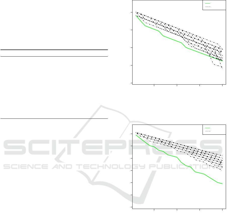
occurs. Thanks to the randomization effect during
Balance call, the performance of different runs is vari-
able. Figures 1, 2 and 3 show the score of Greedy
(solid line) and the scores of 30-runs of Balance
(dashed lines) versus Main with N
1
= N
2
= 30, r = 6,
α = 0.5. The score for the different heuristics is ex-
pressed as a function of the budget B. Red point’s
abcissa is the cost reached by Main after removing 20
nodes. Runs were made on a computer Dell Inspiron-
N4010 with 1.8 GiB of memory, proccesor Intel Core
i3 CPU M380 @ 2.53 GHz x 4, 64 bit’s OS. CPU
times are 0.924 min. for G
USA
, 1.065 min. for G
FON
and 13.021 min. for G
PEG
.
It can be appreciated that our Main heuristic out-
performs both naive solutions Greedy and Balance,
under all possible budgets. Even though Balance
has a reduced computational cost, its performance
presents a large gap with respect to Greedy heuris-
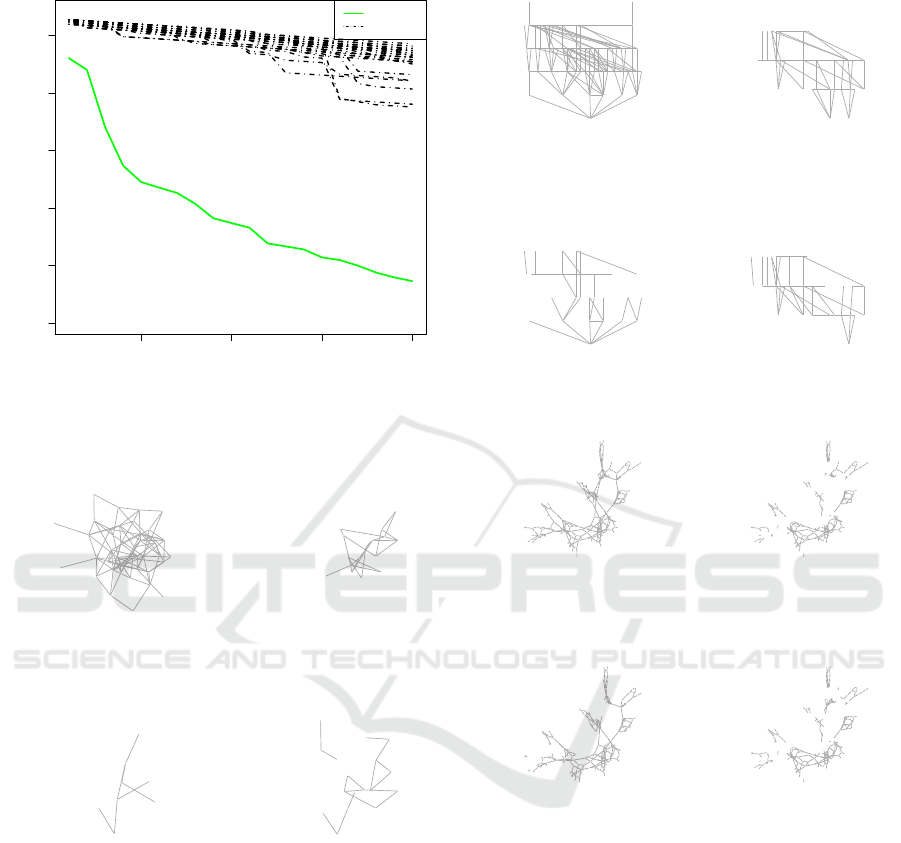
tic. Figures 4, 5 and 6 show the pruning result for the
different heuristics and graphs under study.
5 10 15 20
0 10 20 30 40
Performance Analysis−Neighborhood Graph
Removed nodes
Score
Greedy
Balance
●
Main
Figure 1: Greedy (solid) vs. 30 Balance runs (dashed) for
the Neighborhood Graph.
5 10 15 20
0 10 20 30 40 50 60
Performance Analysis−Fiber Optic Graph
Removed nodes
Score
Greedy
Balance
●
Main
Figure 2: Greedy (solid) vs. 30 Balance runs (dashed) for
the Fiber Optic Graph.
6 CONCLUSIONS
The Graph Fragmentation Problem (GFP) has been
introduced. The goal is to protect (remove) B nodes
from a graph G, in such a way that a random attack to
an arbitrary node v affects the lowest expected num-
ber of nodes (where the whole connected component
from v is affected). The GFP finds applications to fire
fighting, highly virulent epidemic propagations and
electric shocks, among others.
ICORES 2016 - 5th International Conference on Operations Research and Enterprise Systems
142
5 10 15 20
0 50 100 150 200 250
Performance Analysis−IEEE300 Graph
Removed nodes
Score
Greedy
Balance
●
Main
Figure 3: Greedy (solid) vs. 30 Balance runs (dashed) for
the IEEE 300 Graph.
●
●
●
●
●
●
●
●
●
●
●
●
●
●
●
●
●
●
●
●
●
●
●
●
●
●
●
●
●
●
●
●
●
●
●
●
●
●
●
●
●
Neighborhood Graph, Sc= 41
●
●
●
●
●
●
●
●
●
●
●
●
●
●
●
●
●
●
●
●
●
After Greedy, Sc= 12.429
●
●
●
●
●
●
●
●
●
●
●
●
●
After Balance, Sc= 15.571
●
●
●
●
●
●
●
●
●
●
●
●
●
●
●
●
●
●
●
●
●
After Main, Sc= 3.762
Figure 4: Graph G
USA
when α = 1/2.
In this paper, elementary properties of the GFP
were studied. Specifically, graph fragmentation and
balancing are good strategies. Together, they define
a Greedy notion for the problem. Furthermore, we
proved that Greedy achieves improvement in each it-
eration (i.e., in each node protection). A more sophis-
ticated Grasp heuristic enriched with a Path Relinking
post-optimization scheme has been developed. The
effectiveness of our more sophisticated heuristic has
been tested on a real-life networks.
As a future work, we would like to establish the
intractability of GFP and develop different heuristics.
●
● ●
●
●
●
●
● ● ●
●● ● ●
● ●
●
●
●
●●●
●
●
●
●
●
●
●
●
●
●
●
● ●
●
● ●
●
●
●
●●
●
●
●●
●
●
●
●
●
●
● ●
●●
●
●
●
● ●
Fiber Optic Graph, Sc= 62
●
● ● ●
●
●
●
●●
●
●
●
●
●
●
●
●
●
● ● ●
●
●
●
●
●
●●
●
● ●
●
●
● ●
●●
●
●
●
● ●
After Greedy, Sc= 19.095
●
●
●
● ●
●
● ●
●
●
●
●●
●
●
●
●● ●
●
●
●
●
●
● ●
●● ●
●
●
After Balance, Sc= 40.048
● ● ●
●
●
● ● ●
●
●
●
●
●
●
●
●
●
●
● ● ●
●
●
●
●
●
●●
●
● ●
●
●
● ●
●●
●
●
●
● ●
After Main, Sc= 15.524
Figure 5: Graph G
FON
when α = 1/2.
●
●
●
●
●
●
●
●
●
●
●
●
●
●
●
●
●
●
●
●
●
●
●
●
●
●
●
●
●
●
●
●
●
●
●
●
●
●
●
●
●
●
●
●
●
●
●
●
●
●
●
●
●
●
●
●
●
●
●
●
●
●
●
●
●
●
●
●
●
●
●
●
●
●
●
●
●
●
●
●
●
●
●
●
●
●
●
●
●
●
●
●
●
●
●
●
●
●
●
●
●
●
●
●
●
●
●
●
●
●
●
●
●
●
●
●
●
●
●
●
●
●
●
●
●
●
●
●
●
●
●
●
●
●
●
●
●
●
●
●
●
●
●
●
●
●
●
●
●
●
●
●
●
●
●
●
●
●
●
●
●
●
●
●
●
●
●
●
●
●
●
●
●
●
●
●
●
●
●
●
●
●
●
●
●
●
●
●
●
●
●
●
●
●
●
●
●
●
●
●
●
●
●
●
●
●
●
●
●
●
●
●
●
●
●
●
●
●
●
●
●
●
●
●
●
●
●
●
●
●
●
●
●
●
●
●
●
●
●
●
●
●
●
●
●
●
●
●
●
●
●
●
●
●
●
●
●
●
●
●
●
●
●
●
●
IEEE300 Graph, Sc= 265
●
●
●
●
●
●
●
●
●
●
●
●
●
●
●
●
●
●
●
●
●
●
●
●
●
●
●
●
●
●
●
●
●
●
●
●
●
●
●
●
●
●
●
●
●
●
●
●
●
●
●
●
●
●
●
●
●
●
●
●
●
●
●
●
●
●
●
●
●
●
●
●
●
●
●
●
●
●
●
●
●
●
●
●
●
●
●
●
●
●
●
●
●
●
●
●
●
●
●
●
●
●
●
●
●
●
●
●
●
●
●
●
●
●
●
●
●
●
●
●
●
●
●
●
●
●
●
●
●
●
●
●
●
●
●
●
●
●
●
●
●
●
●
●
●
●
●
●
●
●
●
●
●
●
●
●
●
●
●
●
●
●
●
●
●
●
●
●
●
●
●
●
●
●
●
●
●
●
●
●
●
●
●
●
●
●
●
●
●
●
●
●
●
●
●
●
●
●
●
●
●
●
●
●
●
●
●
●
●
●
●
●
●
●
●
●
●
●
●
●
●
●
●
●
●
●
●
●
●
●
●
●
●
●
●
●
●
●
●
●
●
●
●
●
●
After Greedy, Sc= 36.396
●
●
●
●
●
●
●
●
●
●
●
●
●
●
●
●
●
●
●
●
●
●
●
●
●
●
●
●
●
●
●
●
●
●
●
●
●
●
●
●
●
●
●
●
●
●
●
●
●
●
●
●
●
●
●
●
●
●
●
●
●
●
●
●
●
●
●
●
●
●
●
●
●
●
●
●
●
●
●
●
●
●
●
●
●
●
●
●
●
●
●
●
●
●
●
●
●
●
●
●
●
●
●
●
●
●
●
●
●
●
●
●
●
●
●
●
●
●
●
●
●
●
●
●
●
●
●
●
●
●
●
●
●
●
●
●
●
●
●
●
●
●
●
●
●
●
●
●
●
●
●
●
●
●
●
●
●
●
●
●
●
●
●
●
●
●
●
●
●
●
●
●
●
●
●
●
●
●
●
●
●
●
●
●
●
●
●
●
●
●
●
●
●
●
●
●
●
●
●
●
●
●
●
●
●
●
●
●
●
●
●
●
●
●
●
●
●
●
●
●
●
●
●
●
●
●
●
●
●
●
After Balance, Sc= 227.408
●
●
●
●
●
●
●
●
●
●
●
●
●
●
●
●
●
●
●
●
●
●
●
●
●
●
●
●
●
●
●
●
●
●
●
●
●
●
●
●
●
●
●
●
●
●
●
●
●
●
●
●
●
●
●
●
●
●
●
●
●
●
●
●
●
●
●
●
●
●
●
●
●
●
●
●
●
●
●
●
●
●
●
●
●
●
●
●
●
●
●
●
●
●
●
●
●
●
●
●
●
●
●
●
●
●
●
●
●
●
●
●
●
●
●
●
●
●
●
●
●
●
●
●
●
●
●
●
●
●
●
●
●
●
●
●
●
●
●
●
●
●
●
●
●
●
●
●
●
●
●
●
●
●
●
●
●
●
●
●
●
●
●
●
●
●
●
●
●
●
●
●
●
●
●
●
●
●
●
●
●
●
●
●
●
●
●
●
●
●
●
●
●
●
●
●
●
●
●
●
●
●
●
●
●
●
●
●
●
●
●
●
●
●
●
●
●
●
●
●
●
●
●
●
●
●
●
●
●
●
●
●
●
●
●
●
●
●
●
●
●
●
●
●
●
After Main, Sc= 35.343
Figure 6: Graph G
PEG
when α = 1/2.
REFERENCES
Amaldi, E., Capone, A., and Malucelli, F. (2003a). Plan-
ning UMTS base station location: Optimization mod-
els with power control and algorithms. IEEE Transac-
tions on Wireless Communications, 2(5):939–952.
Amaldi, E., Capone, A., Malucelli, F., and Signori, F.
(2003b). Optimization models and algorithms for
downlink UMTS radio planning. In Wireless Com-
munications and Networking, (WCNC’03), volume 2,
pages 827–831.
Borgatti, S. (2006). Identifying sets of key players in a so-
cial network. Computational & Mathematical Orga-
nization Theory, 12:21–34.
Canuto, S., Resende, M., and Ribeiro, C. (2001). Lo-
Graph Fragmentation Problem
143

cal search with perturbation for the prize-collecting
Steiner tree problems in graphs. Networks, 38:50–58.
Dorigo, M. (1992). Optimization, Learning and Natural
Algorithms. PhD thesis, DEI Politecnico de Milano,
Italia.
Feo, T. A. and Resende, M. G. C. (1989). A probabilistic
heuristic for a computationally difficult set covering
problem. Operations Research Letters, 8(2):67 – 71.
Gendreau, M. and Potvin, J.-Y. (2010). Handbook of Meta-
heuristics. Springer Publishing Company, Incorpo-
rated, 2nd edition.
Glover, F. (1989). Tabu search - part i. INFORMS Journal
on Computing, 1(3):190–206.
Goldberg, D. E. (1989). Genetic Algorithms in Search, Op-
timization and Machine Learning. Addison-Wesley
Longman Publishing Co., Inc., Boston, MA, USA, 1st
edition.
Hansen, P. and Mladenovic, N. (2001). Variable neighbor-
hood search: Principles and applications. European
Journal of Operational Research, 130(3):449–467.
Kennedy, J. and Eberhart, R. (1995). Particle swarm opti-
mization. In Proceedings of the IEEE International
Conference on Neural Networks, volume 4, pages
1942–1948. IEEE.
Kirkpatrick, S. (1984). Optimization by simulated an-
nealing: Quantitative studies. Journal of Statistical
Physics, 34(5):975–986.
Lin, S. and Kernighan, B. W. (1973). An Effective Heuristic
Algorithm for the Traveling-Salesman Problem. Op-
erations Research, 21(2):498–516.
Monma, C. L., Munson, B. S., and Pulleyblank, W. R.
(1990). Minimum-weight two-connected spanning
networks. Mathematical Programming, 46(1-3):153–
171.
Ortiz-Arroyo, D. (2010). Discovering sets of key players
in social networks, in Computational Social Network
Analysis, Chp. 2. Springer London.
Papadimitriou, C. H. and Steiglitz, K. (1982). Com-
binatorial optimization: algorithms and complexity.
Prentice-Hall, Inc., Upper Saddle River, NJ, USA.
Resende, M. G. C. and Ribeiro, C. C. (2003). Greedy Ran-
domized Adaptive Search Procedures. In F. Glover
and G. Kochenberger, editors, Handbook of Metha-
heuristics, Kluwer Academic Publishers.
Resende, M. G. C. and Ribeiro, C. C. (2014). Grasp:
Greedy randomized adaptive search procedures. In
Burke, E. K. and Kendall, G., editors, Search Method-
ologies, pages 287–312. Springer US.
Robledo Amoza, F. (2005). GRASP heuristics for Wide
Area Network design. PhD thesis, INRIA/IRISA, Uni-
versit
´
e de Rennes I, Rennes, France.
Romero, P. (2012). Mathematical analysis of schedul-
ing policies in Peer-to-Peer video streaming networks.
PhD thesis, Facultad de Ingenier
´
ıa, Universidad de la
Rep
´
ublica, Montevideo, Uruguay.
Srinivasan, A., Ramakrishnan, K., Kumaram, K., Arava-
mudam, M., and Naqvi, S. (2000). Optimal design
of signaling networks for Internet telephony. In Pro-
ceedgins of the IEEE INFOCOM 2000.
Stoer, M. (1993). Design of Survivable Networks. Lecture
Notes in Mathematics. Springer.
ICORES 2016 - 5th International Conference on Operations Research and Enterprise Systems
144
