Fence Patrolling with Two-speed Robots

Jurek Czyzowicz

, Konstantinos Georgiou

, Evangelos Kranakis

, Fraser MacQuarrie

and Dominik Pajak

Departemant d’Informatique, Universite du Quebec en Outaouais, Gatineau, Qu

ebec, Canada

Department of Mathematics, Ryerson University, Toronto, Ontario, Canada

School of Computer Science, Carleton University, Ottawa, Ontario, Canada

Department of Computer Science FFPT, Wroclaw University of Technology, Wroclaw, Poland

Keywords:

Idleness, Mobile Robots, Patrolling, Speed, Walking, Scheduling.

Abstract:

A fence is to be patrolled collectively by n robots. At any moment a robot may move in one of the two possible

states: walking or patrolling. Each state is associated with a maximal moving speed which cannot be exceeded.

We want to schedule the perpetual movements of the robots so as to minimize the idleness, deﬁned as the

smallest time interval within which every point is always visited by some robot. First, we give a centralized

algorithm constructing schedules with optimal idleness, and subsequently we show an interesting application

to a transportation problem concerning Scheduling with Regular Delivery. Our main contribution is the study

of distributed, dynamical schedules for patrolling robots with only primitive capabilities. Surprisingly, we are

able to design a dynamic schedule for very weak collections of two robots (silent, oblivious, passively mobile),

achieving the optimal idleness. Part of our contribution is a very technical analysis of the dynamics of special

families of dynamical systems of n robots that we call regular. For such systems we also propose a highly

non-trivial O(n

) algorithm to decide whether or not robots converge to a stable conﬁguration thus verifying

if the dynamic schedule is optimal.

1 INTRODUCTION

Fence patrolling is the act of perpetual monitoring of

a domain, modelled as a unit segment, by a set of mo-

bile robots. As the robots cannot continuously moni-

tor all points of the domain, a standard efﬁciency mea-

sure of patrolling is the notion of idleness - the size of

the minimal time interval for which all points of the

domain are always visited (independently of the start

of this interval). Patrolling algorithms attempt to pro-

duce the schedules, (i.e. the trajectories of the robots

in time) minimizing idleness.

In previous research, the robots were supposed

to have either the same or different maximal speeds

of their patrolling movements. In this paper we as-

sume that the patrolling activity requires more elabo-

rate work than just walking within the domain, e.g.,

when foraging or harvesting which take longer than

walking, and in computing applications, web page in-

dexing, forensic search, code inspection, packet sniff-

ing which require a more involved inspection. Conse-

quently, we assume the maximal patrolling speeds to

be strictly smaller than the maximal walking speeds.

We suppose that each robot is capable of pa-

trolling in only one direction (arbitrarily chosen) of

the segment while walking is permitted in both direc-

tions. It is worth noting that the fence problem for

robots patrolling in both directions appears to be quite

difﬁcult. Indeed, optimal idleness algorithms were

found only for fence patrolling of up to three robots,

(cf.(Czyzowicz et al., 2011; Dumitrescu et al., 2014;

Kawamura and Kobayashi, 2012)). Such one-way pa-

trolling assumption is natural for humans, e.g. in text

inspection (cf. the difﬁculty of the backward spelling

game). Several mechanical devices operate actively

in one direction only, e.g. combine and forage har-

vesters, snow-plowers. Also traveling up the hill,

swimming against river ﬂow, carrying heavy loads -

all these activities require slower operating speeds.

We solve optimally the patrolling problem in the

centralized scenario. We also show how to apply our

algorithm to natural optimization problem in trans-

portation concerning Scheduling with Regular Deliv-

ery. Next, and more surprisingly, using a very weak

Czyzowicz, J., Georgiou, K., Kranakis, E., MacQuarrie, F. and Pajak, D.

Fence Patrolling with Two-speed Robots.

DOI: 10.5220/0005687102290241

In Proceedings of 5th the Inter national Conference on Operations Research and Enterprise Systems (ICORES 2016), pages 229-241

ISBN: 978-989-758-171-7

229

collection of mobile robots with only primitive capa-

bilities, we are able to design a distributed strategy

converging to the same optimal solution thus achiev-

ing the same idleness as the optimal centralized al-

gorithm. Our robots are anonymous, oblivious, silent

(no communication permitted) and they cannot pro-

cess any information, as well as they are not aware of

their numbers or their speeds. They are subject to pas-

sive mobility, i.e. their movement is dynamically con-

trolled by their contacts with the environment. The

robots are only capable of walking or patrolling with

maximal speed and their perception mechanism per-

mits only to recognize a collision with the environ-

ment (i.e. the endpoints of the segment or another

robot). This is the ﬁrst study of the patrolling problem

in a decentralized setting thus leading to the design of

a distributed, self-stabilizing algorithm (cf (Dijkstra,

1982)[EWD386, pp 34-35], which discusses a solu-

tion to a cyclic relaxation problem).

1.1 Related Work

Patrolling is the act of surveillance, consisting of

walking perpetually around an area in order to pro-

tect or supervise it, and has been studied intensively

in robotics (Almeida et al., 2004; Chevaleyre, 2004;

Elmaliach et al., 2009; Elmaliach et al., 2008; Hazon

and Kaminka, 2008; Machado et al., 2002; Yanovski

et al., 2003) where it is often viewed as a version

of terrain coverage, a central task in robotics. It is

useful in ecological monitoring, detecting intrusion,

monitoring and locating objects or humans (that may

need to be rescued from a disaster), detecting net-

work failures or even discovering web pages which

need to be indexed by search engines (Machado et al.,

2002). Boundary and area patrolling have been stud-

ied in (Agmon et al., 2008; Elmaliach et al., 2009;

Elmaliach et al., 2008; Pasqualetti et al., 2010; Hare

et al., 2015) with approaches placing more emphasis

on experimental results.

Idleness is the accepted measure of algorithmic ef-

ﬁciency of patrolling and is related to the frequency

with which the points of the environment are visited

(Almeida et al., 2004; Alpern et al., 2011; Cheva-

leyre, 2004; Elmaliach et al., 2009; Elmaliach et al.,

2008; Machado et al., 2002)) (this last criterion was

ﬁrst introduced in (Machado et al., 2002)). Diverse

approaches to patrolling based on idleness criteria are

discussed in (Almeida et al., 2004). Patrolling as a

game between patrollers and intruder is studied in

(Alpern et al., 2009; Alpern et al., 2011; Amigoni

et al., 2010). Elsewhere patrolling is studied based on

swarm or ant-based algorithms (Elor and Bruckstein,

2010; Marino et al., 2009; Yanovski et al., 2003).

Robots are memoryless (or having small memory),

decentralized (Marino et al., 2009) with no explicit

communication permitted either with other robots or

the central station, and may have local sensing capa-

bilities (Elor and Bruckstein, 2010). Ant-like algo-

rithms usually mark the visited nodes of the graph

and (Yanovski et al., 2003) presents an evolutionary

process. This paper shows that a team of memoryless

robots, by leaving marks at the nodes while walking

through them, after relatively short time stabilizes to

the patrolling scheme in which the frequency of the

traversed edges is uniform to a factor of two (i.e., the

number of traversals of the most often visited edge

is at most twice the number of traversal of the least

visited one).

Theoretical graph-based approaches to patrolling

can be found in (Chevaleyre, 2004). In (Pasqualetti

et al., 2010), polynomial-time patrolling solutions

for lines and trees are proposed. For the case of

cyclic graphs, (Pasqualetti et al., 2010) proves the NP-

hardness of the problem and a constant-factor approx-

imation is proposed.

Optimal patrolling with same-speed robots in

mixed domains, where regions to be traversed are

fragmented by components that do not need to be

monitored, is studied in (Collins et al., 2013). Pa-

trolling with robots that do not necessarily have iden-

tical speeds offers several surprises both in terms of

the difﬁculty of the problem as well as in terms of

the algorithmic results obtained. Such a study has

been initiated in (Czyzowicz et al., 2011) and inves-

tigated further in (Dumitrescu et al., 2014; Kawa-

mura and Kobayashi, 2012). The partition strategy,

where each robot patrols and walks along a separate

area, has been proven to work for two robots in (Czy-

zowicz et al., 2011), and for three in (Kawamura and

Kobayashi, 2012).

Standard capabilities of mobile robots usually in-

clude communication, computation, and environment

perception. For many reasons (e.g. production cost,

limited or speciﬁc applications) one may wish to deal

with robots of reduced ability, especially if they are

needed in large numbers. In such cases, feasibility

issues, rather than computation efﬁciency are sought

(Angluin et al., 2006; Angluin et al., 2007; Beauquier

et al., 2010; Cieliebak et al., 2012). (Angluin et al.,

2006) introduced population protocols (see also (An-

gluin et al., 2007; Beauquier et al., 2010)), where

robots are subject to passive mobility, also used in our

paper. Passive mobility aims to model volatile envi-

ronments like water ﬂow, wind or unstable mobility

of agents’ carriers. Further, (Beauquier et al., 2010)

considered different speed of such agents. (cf. also

(Czyzowicz et al., 2013)).

ICORES 2016 - 5th International Conference on Operations Research and Enterprise Systems

230

1.2 Our Model, Problem Deﬁnition &

Notation

Consider a set R of n mobile robots r

,... ,r

each

associated with some patrolling speed p

and some

walking speed w

, where p

< w

for i, j = 1,...,n.

Robots perpetually move along the unit segment [0,1]

in both directions. At any moment, a robot r

may

be in a walking state in which it moves at its walking

speed w

or in the patrolling state and moving at its

patrolling speed p

. Each robot may walk in both di-

rections but its patrolling is always done in the same

direction of the interval [0,1]. Hence we can say that

each robot is associated with its patrolling direction

(positive or negative direction of the interval) which

does not change throughout its entire movement.

The Fence Patrolling Problem: Let S denote a pa-

trolling schedule, i.e. an algorithm associated with

each of the robots dictating on what speed and in

what direction every robot moves at each moment of

time. Given a schedule produced by algorithm A, the

idle time I

(P,t) of a point P at time t is deﬁned as

the amount of time needed to the next visit of P af-

ter time t by any robot of R: I

(P,t) = min{t

> t :

∃i(0 ≤ i ≤ n such that r

) = P)}−t, where we de-

note by r

(t) the point of the segment visited by r

time t, for t ∈ [0,∞). We are interested in an algo-

rithm minimizing the maximal idle time taken over

all points P and all time moments t. However, as

it may be impossible to design an algorithm which

achieves the best possible idle time right from the start

of the schedule (e.g. robots may be in an unsuitable

position to achieve this) we will be allowing any ﬁ-

nite delay for checking idle times of segment points.

More exactly, the idleness of algorithm A is deﬁned as

= inf

T ≥0

sup

0≤p≤1

(P,T ). An optimal patrolling

algorithm is a schedule which optimizes the idleness

among all possible patrolling algorithms under con-

sideration.

It will be useful to observe that our goal may

be viewed as the following equivalent maximization

task. Suppose that the robots operate in an inﬁnite

line. What is the maximal length segment [0, L] and

the perpetual movement of the robots of R, such that

in each unit time interval [t,t + 1] each point of [0, L]

is visited at least once by a robot in patrolling state.

We call such a length L the patrolling range of R.

The Distributed Model: In this model, robots have

only very primitive capabilities allowing them to ex-

ecute separate schedules which change according to

their perception of the environment. They are oblivi-

ous and silent (cannot communicate) and they cannot

process any information. Besides two-speed mobil-

ity they can perceive the environment by recognizing

obstacles (i.e., endpoints) or other robots that they do

not even need to recognize. They are not aware of

their patrolling or walking speeds nor of the length

of the segment. In the schedules produced by our

distributed algorithms the robots function according

to the bouncing-rule: if a robot collides with another

robot or a segment endpoint, then it changes direction

as well as moving-state. A patrolling schedule of n

robots is in a stable conﬁguration (x

∗

,. .. ,x

∗

) if robot

i moves within the interval [x

∗

i−1

∗

] (we set x

∗

= 0

and x

∗

= 1), bouncing always at its endpoints.

Scheduling with Regular Delivery: Our tech-

niques allow us to solve the following transportation

problem. Suppose that at point 1 of the unit segment

there is an inﬁnite quantity of a commodity that is

transported to point 0 by robots R. Each robot may

carry one item of the commodity using a speed not ex-

ceeding p

or it may travel with no load with a speed

not exceeding w

. At any time a robot r

may drop the

item it is carrying at the point currently occupied by

or it may pick up an item present at its current posi-

tion. In particular, when two robots meet at a point an

item being carried by one of them may be transferred

to the other one. At all times no robot may carry more

than one commodity item. What is the smallest value

I, such that during any time interval (kI, (k + 1)I] a

new item is delivered to point 0.

1.3 Our Contributions & Organization

of the Paper

We attempt to solve the Fence Patrolling Problem us-

ing centralized or distributed algorithms. As a warm-

up, we give in Section 2 an optimal centralized al-

gorithm for the problem, whose solution serves as a

benchmark for subsequent sections. We conclude in

Section 2.2 with an interesting application to an opti-

mization transportation problem. Our main technical

contributions appear in Section 3 where we study the

Fence Patrolling Problem in a distributed setting and

where robots have only primitive capabilities. First,

in Section 3.1 we optimally solve Fence Patrolling

with 2 primitive robots. In the same section, we also

develop the main ideas we built upon for patrolling

with an arbitrary number of robots. Then, in Sec-

tion 3.2 we introduce a generic distributed solution

for patrolling with primitive robots. Our solution in-

duces a complex dynamical system, whose analysis is

the main focus of the remaining of the sections. Sec-

tion 3.3 proposes a technical and highly non-trivial

analysis of the dynamics of primitive robots, and con-

Fence Patrolling with Two-speed Robots

231

cludes with an efﬁcient and analytic algorithm for

deciding whether the system of robots converges to

an optimal solution. Finally, Section 3.4 studies re-

stricted, yet natural families of primitive robot col-

lections that have the potential of inducing dynamic

systems that converge to stable and optimal solutions.

With non-trivial and technical arguments, we con-

clude by showing that special families of three and

four primitive robots do solve the Fence Patrolling

problem optimally.

2 OPTIMALLY SOLVING FENCE

PATROLLING BY

CENTRALIZED ALGORITHMS

In this section we give the general, centralized al-

gorithm generating optimal patrolling schedules for

the Fence Patrolling Problem and for any number of

robots.

2.1 Schedule Obtained by a Centralized

Algorithm

Consider the schedule deﬁned by Algorithm 1. The

Algorithm 1: Centralized Schedule.

Input: Set of robots R with associated walking and

patrolling speeds

Output: Schedule of R

1: Let σ

∑

i=1

1/p

+1/w

for j = 1,. .. ,n

2: for j = 1,...,n do

3: Place robot r

at initial position x

= σ

/σ

4: repeat forever

5: In patrolling state, move (left) at speed p

until reaching point x

j−1

6: In walking state, move (right) at speed w

until reaching point x

idea of the algorithm is to divide the unit interval into

subsegments, and to make each robot operate only in

the subsegment associated with it. Robot r

is associ-

ated with a subsegment of size proportional to

Each robot zigzags between the endpoints of its sub-

segment patrolling in one direction and walking in the

opposite direction.

Theorem 2.1. Algorithm 1 produces an optimal pa-

trolling schedule.

Before we provide the proof of Theorem 2.1 we

show Lemmata 2.2 and 2.3.

Lemma 2.2. The idleness I

of Algorithm 1 satisﬁes

= 1/

∑

i=1

1/p

+1/w

Proof. As σ

, j = 0, .. ., n, is an increasing se-

quence, each robot r

operates within the subsegment

j−1

], for j = 1,. .. ,n, having interior disjoint with

all other subsegments. Consider any index j and any

point x ∈ [x

j−1

]. Denote by t

∗

a time when r

is in

the patrolling state and r

∗

) = x. Before r

visits x

in patrolling state the next time, it has to traverse from

x to x

j−1

patrolling followed by walking the subseg-

ment [x

j−1

] and patrolling from x

to x. The time

needed for this equals

x −x

j−1

−x

j−1

−x

=(x

−x

j−1

)





∑

i=1

1/p

+1/w

Lemma 2.3. Let D > 1 be the distance patrolled by

robot r

during some time interval. Then in the same

time interval r

must walk distance at least D −1.

Proof. Suppose, by symmetry, that r

can patrol only

in the right-to-left (i.e. negative) direction of the in-

terval. The difference between the initial and the ﬁnal

position of the robot equals to R −L, where L denotes

the sum of the lengths of its left-to-right moves and

R denotes the sum of the lengths of its right-to-left

moves. Observe that R −L ≤1. As the total patrolling

distance is at most R and the total walking distance is

at least L we have the claim of the lemma.

We are now ready to prove Theorem 2.1.

Proof of Theorem 2.1. Consider any algorithm A

and its idleness I

. It is sufﬁcient to show, that for any

ε > 0 there exists a time interval T = [t

∗

+ I

−ε]

during which some point of the segment is not pa-

trolled by any robot. Let κ be an integer such that

κ >

∑

i=1

1/w

1/p

+1/w

∑

i=1

1/p

+1/w

. Consider any time interval K of

size = κI

. We prove that K must contain interval T

with the property from the claim made above.

Let d

denote the distance traversed by r

while

patrolling during interval K. As each point of the seg-

ment must be patrolled at least κ times during time

interval K we have

∑

i=1

≥ κ. By Lemma 2.3 we

have

−1

≤ κI

, hence d

≤

κI

+1/w

1/p

+1/w

. There-

fore κ ≤

∑

i=1

≤κI

∑

i=1

1/p

+1/w

∑

i=1

1/w

1/p

+1/w

and

≥

∑

i=1

1/p

+1/w

−

∑

i=1

1/w

1/p

+1/w

∑

i=1

1/p

+1/w

≥

∑

i=1

1/p

+1/w

−ε

ICORES 2016 - 5th International Conference on Operations Research and Enterprise Systems

232

This proves Theorem 2.1.

Due to Lemma 2.2, it follows that almost all points

of the segment have the same idle time (with the ex-

ception of the endpoints of subsegments which may

be alternately visited by two robots). From Algo-

rithm 1, it follows that each robot r

operates solely

inside a subsegment of size

1/p

+1/w

∑

i=1

1/p

+1/w

for i = 1, .. ., n. By scaling down the consideration to

the idle time of 1 we easily obtain:

Corollary 2.4. The patrolling range of robot r

hav-

ing patrolling speed p

and walking speed w

equals

1/p

+1/w

. The patrolling range of a set of robots

equals the sum of their patrolling ranges.

2.2 Application to Transportation:

Scheduling with Regular Delivery

In this section we show an interesting application of

our previous ﬁndings in Scheduling with Regular De-

livery (see Section 1.2 for the deﬁnition). The fol-

lowing Proposition shows that the idleness of Algo-

rithm 1 is the optimal value for the problem concern-

ing Scheduling with Regular Delivery.

Proposition 2.5. The solution (i.e., the optimal time

interval) of the problem concerning Scheduling with

Regular Delivery for the set of robots R equals I

- the

idleness of Algorithm 1.

Proof. Each robot of Algorithm 1 revisits the left end-

point of its subinterval (and also its right endpoint)

regularly at time intervals of I

. It is then possible

to synchronize robot movements so that each robot

gets to its subsegment left endpoint (or right endpoint)

exactly at the same when arrives there the left (resp.

right) neighbouring robot. Suppose that robot r

picks

up an item at each visit to point 1 of the segment, and

that, each time a robot reaches the left endpoint of

its subinterval, it transfers the carried item to its left

neighbour. Then each robot r

either walks left-to-

right unload with speed w

or transports one item trav-

eling right-to-left. Consequently, r

delivers one new

item to point 0 at regular time intervals I

. The opti-

mality follows by the argument similar to that used in

the proof of Theorem 2.1.

3 FENCE PATROLLING WITH

PRIMITIVE ROBOTS / THE

DISTRIBUTED CASE

In this section we consider the case when the collec-

tion of patrolling robots acts in a distributed way (see

Section 1.2 for the model). We are interested in an

algorithm having the same idleness as the one of the

optimal centralized algorithm even if our robots are

very weak. For notational reference we will assume

that there exist two motionless robots r

and r

n+1

(i.e.

= p

= w

n+1

= p

n+1

= 0), positioned at the left

and right endpoint, respectively. This way every robot

, for i = 1, .. ., n, bounces at its left or right neighbor.

We have the following lemma.

Lemma 3.1. For any collection R of robots there

exists a centralized algorithm producing an optimal

schedule in stable conﬁguration, in which the robots

behave according to the bouncing rule.

Proof. Consider the partition of the unit interval as in

line 1 of Algorithm 1. By Corollary 2.4 each robot

executing Algorithm 1, within the same time inter-

val, independently covers a segment subinterval pro-

portional to its patrolling range. It is then possible

to reschedule the robots’ starting times so that each

robot arrives at the left endpoint of its subinterval ex-

actly at the same time as when its left neighbor ar-

rives at the right endpoint of its interval, resulting in a

meeting.

We will attempt to design a distributed algorithm

producing robots trajectories converging to a schedule

of a stable conﬁguration of robots. The task seems of

special interest, given that robots are assumed to be

oblivious and silent.

3.1 Distributed Optimal Schedule for

Two Robots

The purpose of this section is to demonstrate that two

primitive robots can optimally solve the Fence Pa-

trolling Problem.

Let I

opt

be the optimal idleness of the ofﬂine

schedule for two robots. We design an algorithm, for

which for any ε > 0 there exists a time t

∗

, such that

in every time interval [t,t + I

opt

+ ε], with t ≥t

∗

, each

point of the segment is visited by some robot. Ob-

viously, using such weak robots, it is impossible to

design an algorithm which achieves optimal idle time

only after some ﬁnite time of their operation. This

would need robots capable of recognizing the param-

eters of the environment (e.g. patrolling and walk-

ing speeds of robots, distance traveled, time between

collisions, etc.). Since robots react only when collid-

ing with each other, or when they reach one endpoint

(as if they do not know when collisions will occur or

where the endpoints are) we slightly abuse standard

terminology and we call our algorithm online.

We show that Algorithm 2 is the optimal one, i.e.

its idleness equals the idleness of the optimal ofﬂine

Fence Patrolling with Two-speed Robots

233

Algorithm 1. The ﬁrst critical observation is that col-

lision points converge to a stable conﬁguration.

Algorithm 2: Online Schedule for Two Robots.

Input: Two robots r

placed at the two segment

endpoints

Output: Schedule of R

1: Both robots start in patrolling state moving to-

wards each other.

2: Each robot switches state and direction when col-

liding either with the other robot or with an end-

point.

Lemma 3.2. The sequence of collision points of Al-

gorithm 2 converges to the point

Proof. Suppose that the two robots following the

schedule produced by Algorithm 2 meet at a point x,

0 < x < 1. Suppose also that before the meeting both

robots were in the patrolling state and moving towards

each other. We show ﬁrst that the next meeting occurs

at a point x

such that

= −

x +

(1)

Indeed, as p

< w

and p

< w

no robot can

be caught from behind by another one, while walk-

ing along the segment. Consequently, both robots

reach the segment endpoints and they restart pa-

trolling while moving towards each other, eventu-

ally colliding at x

. As both robots spend the same

Figure 1: Two robots r

start by patrolling in opposite di-

rections. They ﬁrst collide at a point x and they both change

to walking. After bouncing (not necessarily at the same

time) at the endpoints of the interval [0,1] they change to

patrolling and meet anew at point x

. The vertical line indi-

cates time.

time while traveling from x to x

(cf. Figure 1) we

have

1−x

. Therefore x





−x





. We see from Identity (1)

that x

= −Ax + B where

A :=

,B :=

. (2)

If x

is the initial collision point then we see that

the kth collision point satisﬁes the recurrence x

−Ax

k−1

+ B. This yields a geometric series from

which it follows that x

= (−A)

1−(−A)

1+A

. Since

A < 1 as k → ∞ we get x

→

1+A

which completes the proof.

Our intention is to generalize the lemma above for

dynamic systems with arbitrarily many robots. Till

then, we show that Algorithm 2 produces the optimal

schedule.

Theorem 3.3. The idleness of the schedule of Algo-

rithm 2 equals I

- the idleness of the optimal schedule

produced by the centralized algorithm.

Proof. It is sufﬁcient to show that for any ε > 0 there

exists a point in time t

∗

such that for any t > t

∗

and

any time interval T = [t,t + I

+ ε] each point of the

segment is patrolled by some robot. Observe that

from the start to the ﬁrst meeting point x

robot r

patrols the interval [0,x

], while during the same time

interval r

patrols the interval [x

,1]. Hence we have

1−x

. Solving for x

we get x





Observe that the distance D = |x

−x

k−1

| between

the (k −1)-th and k-th meeting points (deﬁned in the

proof of Lemma 3.2)

D =





(−A)

+ B

1−(−A)

1+A



−



(−A)

k−1

+ B

1−(−A)

k−1

1+A





((−A)

−(−A)

k−1

)(x

−

1 + A

)



= |(−A)

(B −x

(A + 1))|

= A

(B −x

(A + 1))

(since A > 0 & (B −x

(A + 1)) > 0)

is converging to 0, since |A| < 1. As x

and x

k−1

are

on the different sides of the convergence point

1+A

within every time interval I

min(p

)

the entire

segment is jointly patrolled by both robots. Let K

be such that K ≥ log

ε·min(p

)

B−x

(A+1)

and let t

∗

> (K +

1)(

). As (

) is

the time between two consecutive bounces between

robots r

, after time t

∗

the robots bounced at least

k times. Hence (as 0 < A < 1) for t > t

∗

the idle time

I(p,t) of every point p is I(p,t) ≤ I

min(p

)

ICORES 2016 - 5th International Conference on Operations Research and Enterprise Systems

234

(B−x

(A+1))

min(p

)

≤I

+ε, which proves the theorem.

Observe that Algorithm 2 works even if the robots

do not necessarily start their respective schedules at

the same time. Indeed, because p

< w

, i, j = 1,2,

when the second robot wakes up and starts patrolling

it cannot meet the robot which started ﬁrst while this

robot is in the walking state. Therefore the robots

meet when they are both in the patrolling state and

the subsequent meetings converge to the same point

as before.

Note that, when robots start walking rather than

patrolling, their subsequent meeting points do not

converge.

On the other hand if one robot starts in

the walking state while the other one in the patrolling

state the convergence is possible in at most one of

the two symmetric cases, depending which among the

two values 1/p

+ 1/w

or 1/w

+ 1/p

is larger. In

particular, when 1/p

+ 1/w

= 1/w

+ 1/p

(e.g. in

the case of identical robots) the meeting points alter-

nate between two symmetric positions on the segment

and the idleness is clearly suboptimal (cf. Fig. 2).

(0)

= x

(2)

(1)

Figure 2: Two robots r

perpetually alternate between

x(0) and x(1) (r

starts by patrolling and r

by walking).

Here w

= 5, p

= 3

= 10, p

= 4.

3.2 Distributed Schedule for n Primitive

Robots

In this section we propose a distributed solution for

an arbitrary number of primitive robots that induces

an interesting dynamic system, which we analyze in

subsequence sections.

As observed for the case of two robots, the conver-

gence was attested if the two robots were colliding al-

ways in the patrolling state. For more than two robots

this condition can no longer be guaranteed as all but

two robots collide with both neighbors. We begin our

This follows from the proof of Theorem 3.3, as in this

case, the critical value of quantity A =

1/p

+1/p

1/w

+1/w

> 1 (the

roles of patrolling and walking speeds are swapped in the

equation for x

analysis by proposing Algorithm 3, an intuitive dis-

tributed schedule that assumes the bouncing rule, i.e.

that robots can respond to bounces by ﬂipping their

moving state (e.g. from walking to patrolling) and

their moving direction. Moreover, as in our setting

robots will start walking simultaneously at the same

segment endpoint we naturally assume that p

6= p

(and that w

6= w

), otherwise identical robots would

always stay together and only one of them would con-

tribute to the patrolling algorithm. As all robots pa-

Algorithm 3: Distributed Schedule for Many Robots.

Input: A collection R of robots with distinct pa-

trolling and walking speeds

Output: Schedule of R

1: All robots start from the rightmost endpoint of the

interval, in patrolling state moving right-to-left.

2: Each robot switches state and direction while col-

liding with the other robot or with an endpoint.

trol in the same direction and they change states only

when meeting we can conclude with the following:

Observation 3.4. Algorithm 3 produces a dynamic

schedule with Regular Delivery, for a given set of

robots.

Notice that our algorithm deﬁnes a complex dy-

namical system of memoryless robots moving back

and forth in an interval. The analysis of the system

dynamics is very complicated, given that robot col-

lisions might occur either between robots moving in

opposite directions, or in the same directions (i.e. a

collision may happen from behind). In what follows

we analyze the dynamics under the assumption that

we have one type of collisions, which as we shall see

in the next subsections naturally arise by restricting

the conﬁguration of the robot speeds to what we later

call monotone speeds.

We call the dynamical system that arises from Al-

gorithm 3 regular if collisions occur only between

robots that move in opposing directions, and there-

fore collisions happen only between a robot that is

in patrolling state moving right-to-left and a robot in

walking state moving left-to-right. We are interested

in answering whether regular dynamical systems con-

verge in a stable conﬁguration, and whether this con-

ﬁguration has optimal idle time. Below we propose

a highly efﬁcient algorithm for verifying whether a

regular dynamical system has this property (for any

number of robots). Then we answer this question in

the positive for up to 4 robots, under the assumption

that speeds satisfy a natural condition.

Fence Patrolling with Two-speed Robots

235

3.3 Dynamics for Regular Systems of

Primitive Robots

Dynamic systems of primitive robots induced by Dis-

tributed Algorithm 3 are highly complex and difﬁcult

to analyze. The purpose of this section is to provide a

deep and technical analysis of the dynamics of regu-

lar systems. We conclude the section by proposing a

highly non-trivial algorithm for deciding convergence

of primitive robots in a stable conﬁguration (where

robots eventually move in disjoint subintervals).

Notice that in every dynamical system, and at ev-

ery point in the time horizon, robots will appear on

the interval in the same order. We rename the robots

so that robot i+1 is always to the right of robot i, after

they develop according to Algorithm 3. Below we de-

note by x

the point in the interval where robots r

i+1

bounce for the t-th time. The purpose of the next

lemma is to predict points x

. The reader may view

it as the analogue of (part of the proof of) Lemma 3.2

that dealt with only two robots.

Lemma 3.5. In a regular system we have



i+1



t+1

−





i−1

t+1



i+1



i+1

−



i+1



Proof. First we claim that x

i−1

< x

, i = 1,. .. ,n,

and that robots r

i−1

bounce at x

i−1

before r

i+1

bounce at x

. Indeed, let τ(x

) denote the time of this

bounce. Note that robot r

(while patrolling) bounces

ﬁrst at the origin and on its way back (now walk-

ing) bounces with robot r

(which is patrolling). Af-

ter robot r

bounces with robot r

, it begins walking

and eventually bounces with robot r

which moves

in opposite direction and is patrolling, etc. This rea-

soning shows that x

i−1

< x

, i = 1,. ..,n as well as

that r

i−1

bounce for the ﬁrst time before r

i+1

do.

Since the system is regular, each robot alternates its

bounces between both neighbors r

i−1

, r

i+1

which is

sufﬁcient to conclude the claim.

Next observe that between time τ(x

) and τ(x

t+1

)

robot r

i−1

ﬁrst patrols right-to-left the interval

i−1

t+1

] then it walks left-to-right the interval

i−1

t+1

]. During the same time interval r

ﬁrst

walks left-to-right the interval [x

i+1

] then it patrols

right-to-left the interval [x

t+1

i+1

] (see Figure 3).

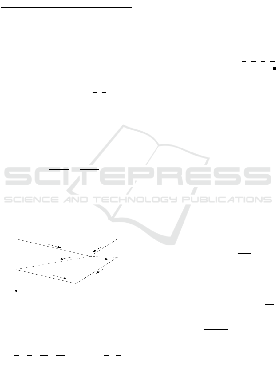
Comparing both times we get

−x

i−1

t+1

−x

i−1

t+1

i+1

−x

i+1

−x

t+1

i+1

. Regrouping terms implies the

lemma.

i+1

i−1

t+1

i+1

Figure 3: Two time consecutive bounces between robots

i+1

We can rewrite the recurrence in Lemma 3.5 in a

more concise matrix form. Deﬁne the following ma-

trices.

A = diag



i+1



i=1,...,n−1

−L-diag





i=2,...,n−1

(3)

B = diag



i+1



i=1,...,n−1

(4)

−U-diag





i=2,...,n−1

(5)



0,. .. ,



where by L-diag and U-diag we mean the low and

upper diagonal matrices of dimension (n −1) ×(n −

1) and entries as indicated placed below and above

the main diagonal, respectively.

Theorem 3.6. Consider a regular dynamical system

of n robots (produced by Algorithm 3) and let A, B,c

be the matrices deﬁned in Equations (4). If the moduli

(norms) of all eigenvalues of the matrix A

−1

B are less

than 1, then the schedule of Algorithm 3 converges to

a schedule in stable conﬁguration which is also opti-

mal (w.r.t. to centralized algorithms). In particular,

for every ε > 0, after Θ (log1/ε) bounces (iterations)

of any pair of neighboring robots the idle time I

(p,t)

is such that I

(p,t) ≤ (1 + ε)

∑

i=1

1/p

+1/w

Proof. Let X

∈ R

n−1

be the vector



,. .. ,x

n−1



Then the recurrence of Lemma 3.5 can be rewritten in

matrix form as AX

t+1

+BX

= c. From this, we derive

that

(−1)



−1





I + A

−1



−1



I −(−1)

−1



−1





−1

Next consider the eigenvalue decomposition A

−1

B =

QΛQ

, where Q is an orthogonal matrix. Then



−1



= QΛ

, and since lim

t→∞

= 0 as all

eigenvalues have norm less than 1, we conclude

ICORES 2016 - 5th International Conference on Operations Research and Enterprise Systems

236

that lim

t→∞

exists, i.e. the sequence converges to

∗



I + A

−1



−1

c = (A + B)

−1

c and the con-

vergence is linear. From the deﬁnition of the recur-

rence, it follows that the schedule of Algorithm 3 con-

verges to the schedule S which is in stable conﬁgura-

tion X

∗

By Corollary 2.4 which, in view of Lemma 3.1,

applies also to stable conﬁgurations the patrolling

range of the collection of robots equals

∑

i=1

1/p

+1/w

and by the rate of convergence, after Θ (log1/ε)

bounces of neighboring robots, the idle time is already

no more than than (1 + ε)

∑

i=1

1/p

+1/w

Note that already Theorem 3.6 suggests a nu-

merical method for checking whether the dynamical

system arising from Algorithm 3 converges or not;

given patrolling and walking speeds p

, ﬁrst com-

pute matrix A

−1

, and then calculate all eigenvalues of

−1

B and verify that their norm is less than 1. Ma-

trix inversing can be done explicitly and efﬁciently,

say by Gauss-Jordan elimination or by LU decompo-

sition. Finding however the eigenvalues of the non-

Hermitian matrix A

−1

B is at least as difﬁcult as ﬁnd-

ing the roots of high degree polynomials. In light

of Abel’s impossibility theorem, one has to rely on

numerical methods to verify that the moduli of the

eigenvalues of A

−1

B are indeed less than 1. In fact,

a number of sophisticated numerical methods have

been proposed to efﬁciently ﬁnd eigenvalues of spe-

cial families of matrices.

We depart from this approach, and in contrast to

numerical methods, we propose an explicit, symbolic

and efﬁcient algorithm for verifying the precondi-

tion of Theorem 3.6 without explicitly computing the

eigenvalues of A

−1

B. Our strategy is to ﬁrst give an

explicit expression of A

−1

, which in turn will allow

us to calculate the characteristic polynomial of A

−1

Finally, we invoke a powerful theorem that charac-

terizes the range of polynomial roots (without ﬁnding

them), and that can be exploited algorithmically.

We begin by calculating the characteristic polyno-

mial of A

−1

B. Note that for a group R of n robots, the

characteristic polynomial of A

−1

B is of degree n −1.

Also, any r ×r leading principal minor A

−1

B can be

computed from the r ×r leading principal minors of

A,B, which only depend on robots 1,. .. ,r +1. In fact

the r ×r leading principal minor A

−1

B is exactly the

critical matrix whose eigenvalues determine the con-

vergence of Algorithm 3 for input robots 1,...,r + 1.

So, we are motivated in denoting by D

(λ) the char-

acteristic polynomial of the r ×r leading principal mi-

nor A

−1

B (i.e. D

n−1

(λ) = |A

−1

B −λI|). We choose

to abbreviate D

(λ) by D

. The next lemma provides

two alternative recursive relations for D

(each will

be convenient in different arguments) that allow us to

compute D

n−1

, and will be also used later to establish

convergence for special cases of robots.

Lemma 3.7. Consider matrices A, B as deﬁned

in (4), and introduce the abbreviations a

i+1

:= −

i+1

−

i+1

, and α

−

i−1

,β

i−1

. Then for the characteristic polyno-

mials D

, the following equivalent recurrences hold

true for all r ≥ 2

= (α

−λ) ·D

r−1

r−2

∑

t=1

t+1

∏

j=t+2

·D

∏

j=2

, (6)



−λ



r−1

λD

r−2

(7)

and with initial conditions D

−λ, D

= 1.

Proof. The inverse of A is a lower triangular matrix

and can be easily veriﬁed to be deﬁned as

−1

i j

:= (−1)

i+ j

∏

i−1

t= j

∏

r= j

, if j ≤ i

and is 0 otherwise. Therefore, for the (so-called

Hessenberg matrix, as it has zero entries above the

ﬁrst subdiagonal) matrix A

−1

B we have that



−1



i j

= (−1)

i+ j

i−1

∏

t= j

−

j−1

∏

t= j

t−1

if i ≥ j −1, and 0 otherwise, with the understanding

that c

= 0. The following interesting relation holds

for the entries of A

−1

B, that is useful in ﬁnding the

characteristic polynomial of the matrix.



−1



i, j

= −

i−1



−1



i−1, j

, ∀i > j. (8)

Next we introduce D

to denote a small variation of

. D

is the determinant of the same principal minor

of A

−1

B −λI (up to entry (r,r)) with the only dif-

ference that the entry (r,r) is replaced by



−1



r,r

instead of



−1

B −λI



r,r

With this notation, we can evaluate



−1

B −λI



by expanding the determinant with respect to the en-

tries (n −1,n −1) and (n −2, n −1). Using Equa-

tion (8), we observe that

−

r−1

−λ

r−1

, (9)

−

r−1

, (10)

Fence Patrolling with Two-speed Robots

237

where the recurrence ends at D

−λ and D

. Repeated substitution of (10) to (9) and some di-

rect calculations imply recurrence (6). Recurrence (7)

is obtained from (6) by subtracting two consecutive

terms of the sequence D

Notice that Lemma 3.7, and in particular Equa-

tion (7), allows us to calculate the characteristic poly-

nomial D

n−1

of A

−1

B by performing no more than

Θ(n

) arithmetic operations (additions, multiplica-

tions and divisions) between speeds p

. Next we

give an efﬁcient algorithm for deciding whether the

moduli of the roots of an arbitrary polynomial f : R 7→

R are all less than 1. Our intention is to run Algo-

rithm 4 with input D

n−1

, i.e. the characteristic poly-

nomial of A

−1

Algorithm 4: Decide Convergence.

Input: A polynomial f : R 7→ R of degree t of the

form

∑

i=0

1: Set γ

(0)

= γ

, for i = 0, .. .,t.

2: For j = 0,...,t −1 and for k = 0, .. ., j + 1 com-

pute γ

( j+1)

= γ

( j)

−γ

( j)

n−j

( j)

n−j−k

3: Compute δ

j+1

:= γ

( j+1)



( j)



−



( j)

n−j



for

j = 0, .. .,t −1.

Output: YES if and only if δ

< 0 and δ

> 0 for

j = 2, .. .,t.

Theorem 3.8. A set of n robots R for which the out-

put of Algorithm 3 gives a regular dynamical system

converges to a stable conﬁguration if and only if Al-

gorithm 4 outputs YES on input D

n−1

. As a result,

convergence can be decided in Θ(n

) arithmetic op-

erations.

Proof. By Theorem 3.6, the regular dynamical sys-

tem converges to a stable conﬁguration if and only

if all eigenvalues of A

−1

B (as deﬁned in (4)) have

moduli less than 1. The characteristic polynomial of

−1

B can be computed in Θ(n

) many operations, as

a corollary of Lemma 3.7. Clearly, Algorithm 3.8

requires no more than Θ(n

) arithmetic operations.

Therefore,we can decide convergence in Θ(n

) arith-

metic operations as long as we can show that Algo-

rithm 4 correctly decides whether the input polyno-

mial f has all its roots (real or complex) strictly inside

the unit circle.

Correctness of Algorithm 4 is an immediate corol-

lary of Theorem 42,1, p. 150 in (Marden, 1949): “Set

∆

∏

j=1

, ,r = 1,. .. ,t and suppose that k many

of the products ∆

are negative, and the remaining

t −k of them are positive. Then f has exactly k roots

strictly inside the unit circle, exactly t −k roots strictly

outside the unit circle (and hence no roots on the unit

circle).”

3.4 Monotone Robot Collections, and

Convergence

In this section we demonstrate some special families

of primitive robots that can solve Fence Patrolling op-

timally. The analysis even of the restricted families of

three or four robots remains surprisingly technical and

non-trivial.

Our technical results of Section 3.3 on regular dy-

namical systems raise the question whether such sys-

tems exist. A natural family of robots is when ei-

ther the sum or the product of patrolling and walking

speeds is constant for all robots or when some con-

stant “power” of a robot may be used for improving

its patrolling ability at the expense of its walking abil-

ity. In such a collection of robots, all patrolling speeds

are dominated by the walking speeds, and the non-

increasing order of patrolling speeds is the inverse or-

der of that of the walking speeds. We make the deﬁ-

nition formal.

Deﬁnition 3.9. The collection R of n robots is called

monotone if for i, j = 1, .. ., n: 1) p

< w

, 2) p

6= p

and 3) p

< p

=⇒ w

> w

A natural example of a monotone collection of

robots is one where each robot i independently de-

cides how to distribute it’s energy e, which is the same

for all robots, to walking and patrolling speeds w

, p

respectively, such that w

+ p

= e. As it is observed

before, a collection of robots that develop according

to Algorithm 3 preserve the order they appear on the

line. Without loss of generality we may assume that

their indices are consecutive along the segment, i.e.

that w

> w

n−1

> ··· > w

> p

> ··· > p

Lemma 3.10. For a monotone collection of robots R,

the dynamical system that arises from Algorithm 3 is

regular (i.e. collisions occur while robots approach

each other, the left one being in the walking state and

the right one in the patrolling state.)

Proof. Initially all robots walk right-to-left until the

fastest walking robot collides with the left endpoint

and starts walking left-to-right. Any “head on” colli-

sion results in the right robot switching to patrolling

left-to-right and the left robot switching to patrolling

right-to-left. So it is sufﬁcient to prove that colli-

sions from behind never take place. Suppose to the

contrary, that there exists such a collision between

a pair of consecutive robots on the segment, r

i+1

for i = 1, .. ., n −1. Obviously r

i+1

cannot collide

when r

moves left and r

i+1

moves right. If both

ICORES 2016 - 5th International Conference on Operations Research and Enterprise Systems

238

robots move right-to-left then, by assumption, they

must be walking, and since w

< w

i+1

, r

cannot catch

i+1

. Similarly, if both robots move left-to-right, by

assumption, they are patrolling and since p

> p

i+1

cannot catch r

As an immediate observation, we also obtain that

< 1 &

i−1

)

i−1

< 1 (11)

for all i = 1,...,n−1 and i = 2,...,n−1 respectively,

and for all regular collections of n robots, where

are as in Lemma 3.7. In fact, the characteristic

polynomial D

n−1

has leading coefﬁcient (−1)

, while

it is also immediate from (7) that the constant coefﬁ-

cient is

∏

n−1

i=1

< 1. This automatically shows that

the condition δ

< 0, of Algorithm 4, holds true for

monotone collections of robots. In fact, we conjec-

ture that monotone collections of robots always con-

verge to a stable conﬁguration, i.e. that δ

> 0 for

j = 2,...,n−1, but a general proof is eluding us. Still

the proof of convergence for up to n ≤3 robots is easy

to establish. The proof of the next proposition relies

on (11).

Proposition 3.11. For a monotone collection of n ≤3

robots the schedule produced by Algorithm 3 has the

optimal idleness.

Proof. We show that the conditions of Theorem 3.6

are satisﬁed. The case of 1 robot is straightforward.

For n = 2 robots, the characteristic polynomial is

−x, which by (11) has one real root with

absolute value less than 1.

Now we turn our attention to n = 3, and by (7)

the characteristic polynomial D

(λ) has the form

(λ) := (U − λ)(V − λ) + W λ = λ

− (U + V −

W )λ +UV , where U,V,W are non negative constants

which by (11) are strictly less than 1.

We show that the moduli of the roots of P

(λ)

are less than 1. First we observe that P

(λ) has this

property.

Case 1: If P

(λ) has real roots, then these are ρ

(W )

1,2

U+V −W±

√

(U+V −W )

−4UV

, with the understanding

that ρ

(W )

,ρ

(W )

correspond to the square root having

positive and negative sign respectively. Then we ob-

serve that ρ

(W )

< ρ

(0)

< 1, while also ρ

(W )

> −W /2 >

−1/2 (by ignoring the positive terms). Hence

−1/2 < ρ

(W )

< 1. Similarly, we see that ρ

(W )

(U +V )/2 < 1 (by ignoring the negative terms). And

ﬁnally note that U + V −

(U +V −W )

−4UV >

−W, since (U + V + W )

> (U + V −W )

−4UV .

Therefore, ρ

(W )

> (−2W )/2 = −1, concluding that

−1 < ρ

(W )

< 1, as well.

Case 2: If P

(λ) has complex roots, say σ

,σ

, then

it must be the case that kσ

= kσ

= σ

UV < 1.

We now prove convergence of monotone collections

of n = 4 robots by using a reﬁnement of monotonicity.

Deﬁnition 3.12. The collection R of n robots is called

strongly monotone if it is monotone and for all r we

have



r+1



r−1







Due to the deﬁnitions of a

and that of α

in Lemma 3.7, asking that a collection of robots is

strongly monotone is equivalent to asking that α

> 0

for every r (see (6)). This allows us to show that char-

acteristic polynomials associated with such robots

have no negative real roots. We can now prove that

the characteristic polynomial of every strongly mono-

tone collection of robots has real roots less than 1 in

absolute value.

Theorem 3.13. For every monotone (not necessarily

strongly) collection of n robots, D

(λ) preserves sign

for all λ ≥ 1. If in addition robots are strongly mono-

tone, then D

(λ) preserves sign (and is actually posi-

tive) for all λ < 0. As a result all real roots of D

lie

strictly between 0 and 1.

Proof. The less technical proof concerns the strongly

monotone collections of robots. For this consider the

cone C of polynomials of the form

∑

t=0

(−1)

where ρ

> 0 , i.e. polynomials whose odd-degree

monomial coefﬁcients are negative, and whose even-

degree monomial coefﬁcient are positive. Clearly, any

polynomial p(λ) ∈ C is positive for every λ < 0 (and

is actually decreasing).

We claim that for all r ≥0, D

∈C . To that end, we

ﬁrst observe that the statement is true for r = 0,1. For

any r ≥ 2, we invoke (6). Since all α

,β

are positive

reals, we can show that D

∈ C as long as we can

verify that (α

−λ) ·D

r−1

∈ C (the rest of summands

in (6) are conical combinations of polynomials in C ).

It is straightforward now to check that −λD

r−1

∈ C ,

hence (α

−λ) ·D

r−1

= α

r−1

+ (−λD

r−1

) ∈ C , as

wanted.

Now we focus on a monotone (not necessarily

strongly) collection of robots. We prove by induction

on r that for all λ ≥ 1, D

is a polynomial which is



positive and increasing, if r is even

negative and decreasing, if r is odd

Indeed, the statement is true for r = 1, 2. Next we

turn our attention to r ≥ 3. We have in mind to in-

voke (7). Now ﬁx any λ

≥ 1. Note that

−λ

< 0.

Next observe that if r is even, then D

r−1

(λ

) < 0 and

r−2

(λ

) > 0, so that D

(λ

) > 0. Similarly, if r is

Fence Patrolling with Two-speed Robots

239

odd, then D

r−1

(λ

) > 0 and D

r−2

(λ

) < 0, so that

(λ

) < 0, exactly as wanted.

Next we show the promised monotonicity. Let’s

denote by D

(λ) the ﬁrst derivative of D

(λ) with re-

spect to λ. Then we see that

(λ) =

−λD

r−1

(λ) +



−λ



r−1

(λ)

r−1

r−2

(λ) +

r−1

λD

r−2

(λ)

If r is even then we argue that D

(λ) > 0 for all

λ ≥ 1. Indeed, we have that

−λD

r−1

(λ) = −·+ ·− = +



−λ



r−1

(λ) = −·− = +

r−1

r−2

(λ) = + ·+ = +

r−1

λD

r−2

(λ) = + ·+ ·+ = +

Since all summands of D

(λ) are positive, D

(λ) is

increasing.

Similarly, if r is odd, we show that D

(λ) < 0 for

all λ ≥ 1. Indeed, we have that

−λD

r−1

(λ) = −·+ ·+ = −



−λ



r−1

(λ) = −·+ = −

r−1

r−2

(λ) = + ·− = −

r−1

λD

r−2

(λ) = + ·+ ·− = −

Since all summands of D

(λ) are negative, D

(λ) is

decreasing.

In order to show that a group of strongly monotone

robots converges to a stable conﬁguration, it remains

to prove all complex roots of D

have norm < 1; this

is the main idea behind the proof of Proposition 3.14.

Proposition 3.14. For a strongly monotone collection

of n = 4 robots the schedule produced by Algorithm 3

has the optimal idleness.

Proof of Proposition 3.14. Again, we show that the

conditions of Theorem 3.6 are satisﬁed. When

n = 4, and using (7), we can write the char-

acteristic polynomial we need to study, that has

the form D

(λ) = (A

− λ)(A

− λ) +

λ(B

−λ) + B

−λ)), where by A

we abbre-

viate b

and by B

we abbreviate c

i−1

. Next

we argue that all roots of D

have norm less than 1.

By assuming strong monotonicity, Theorem 3.13 says

that all real roots have norm between 0 and 1. Hence,

we only need to check any complex roots. All we

need to use below is that 0 ≤ A

< 1, and this fol-

lows by assuming simple (speed) monotonicity.

Since D

is of degree 3, it always has a real root,

call it r, and at most two complex roots (that are con-

jugate to each other), say with norm kρk. Since the

constant term of D

is A

, it follows that kρk =

. Next we prove that r ≥min{A

}, con-

cluding what we need. Indeed, consider the polyno-

mial

+ B

(λ)

−λ)(A

−λ)

+λ



−λ) +

−λ)



which clearly has the same roots as D

(λ). Now,

the root r above is a value for λ that satisﬁes

the following equality

−λ)(A

−

λ) = −λ



−λ) +

−λ)



. The

left-hand-side polynomial, which is of degree 3, has

real roots A

, and most importantly it is de-

creasing for all x ≤ min{A

} and for all λ ≥

max{A

}. The right-hand-side polynomial is

of degree 2, and has two real roots. One of them

is 0, and the other, call it r, is a convex combina-

tion of A

, hence we have min{A

} ≤ r ≤

max{A

}. Moreover, the degree 2 polynomial

is negative for 0 < λ < r and positive for λ > r,

and is increasing for all λ ≥ r. Since r is in the

line segment between min{A

},max{A

}, it

must be the case that the graphs of the two polyno-

mials intersect for some λ between min{A

}

and max{A

}.Therefore, r ≥ min{A

}

as wanted.

4 CONCLUSION

Patrolling a given domain with a swarm of two-speed

robots is a challenging problem with interesting trade-

offs. Its difﬁculty, even for patrolling a segment, is

due to the fact that there are many patrolling strate-

gies to be taken into account. We gave an optimal

ofﬂine algorithm for any robot collection and opti-

mal dynamic schedules for two robots. We also gave

an efﬁcient algorithm deciding self-stabilization of a

distributed schedule for the case of regular dynamical

systems. We proved that the distributed algorithm is

self-stabilizing for up to four robots whose speeds sat-

isfy a certain monotonicity property. However, con-

vergence of our distributed algorithm for more than

ICORES 2016 - 5th International Conference on Operations Research and Enterprise Systems

240

four robots (whose speeds satisfy a certain mono-

tonicity property) remains open. The case of differ-

ent domains is interesting and can be surprisingly de-

manding.

ACKNOWLEDGEMENTS

For the ﬁrst and third author, this research was sup-

ported in part by NSERC grants.

REFERENCES

Agmon, N., Kraus, S., and Kaminka, G. A. (2008). Multi-

robot perimeter patrol in adversarial settings. In ICRA,

pages 2339–2345.

Almeida, A., Ramalho, G., Santana, H., Tedesco, P. A.,

Menezes, T., Corruble, V., and Chevaleyre, Y. (2004).

Recent advances on multi-agent patrolling. In SBIA,

pages 474–483.

Alpern, S., Morton, A., and Papadaki, K. (2009). Optimiz-

ing randomized patrols. Operational Research Group,

London School of Economics and Political Science.

Alpern, S., Morton, A., and Papadaki, K. (2011). Patrolling

games. Operations research, 59(5):1246–1257.

Amigoni, F., Basilico, N., Gatti, N., Saporiti, A., and

Troiani, S. (2010). Moving game theoretical pa-

trolling strategies from theory to practice: An usarsim

simulation. In ICRA, pages 426–431.

Angluin, D., Aspnes, J., Diamadi, Z., Fischer, M., and Per-

alta, R. (2006). Computation in networks of passively

mobile ﬁnite-state sensors. Distributed Computing,

18(4):235–253.

Angluin, D., Aspnes, J., Eisenstat, D., and Ruppert, E.

(2007). The computational power of population pro-

tocols. Distributed Computing, 20(4):279–304.

Beauquier, J., Burman, J., Clement, J., and Kutten, S.

(2010). On utilizing speed in networks of mobile

agents. In Proceeding of the 29th ACM SIGACT-

SIGOPS Symposium on Principles of distributed com-

puting, pages 305–314. ACM.

Chevaleyre, Y. (2004). Theoretical analysis of the multi-

agent patrolling problem. In IAT, pages 302–308.

Cieliebak, M., Flocchini, P., Prencipe, G., and Santoro,

N. (2012). Distributed computing by mobile robots:

Gathering. SIAM J. Comput., 41(4):829–879.

Collins, A., Czyzowicz, J., Gasieniec, L., Kosowski,

A., Kranakis, E., Krizanc, D., Martin, R., and

Morales Ponce, O. (2013). Optimal patrolling of frag-

mented boundaries. In SPAA.

Czyzowicz, J., Gasieniec, L., Kosowski, A., and Kranakis,

E. (2011). Boundary patrolling by mobile agents

with distinct maximal speeds. Algorithms–ESA 2011,

pages 701–712.

Czyzowicz, J., Kranakis, E., and Pacheco, E. (2013). Lo-

calization for a system of colliding robots. In ICALP

(2), pages 508–519.

Dijkstra, E. W. (1982). Selected writings on computing: a

personal perspective. Springer-Verlag New York, Inc.

Dumitrescu, A., Ghosh, A., and Csaba, D. T. (2014).

On fence patrolling by mobile agents. CoRR,

abs/1401.6070.

Elmaliach, Y., Agmon, N., and Kaminka, G. A. (2009).

Multi-robot area patrol under frequency constraints.

Ann. Math. Artif. Intell., 57(3-4):293–320.

Elmaliach, Y., Shiloni, A., and Kaminka, G. A. (2008). A

realistic model of frequency-based multi-robot poly-

line patrolling. In AAMAS (1), pages 63–70.

Elor, Y. and Bruckstein, A. M. (2010). Autonomous multi-

agent cycle based patrolling. In ANTS, pages 119–

130.

Hare, J., Gupta, S., and Wilson, J. (2015). Decentralized

smart sensor scheduling for multiple target tracking

for border surveillance. In ICRA, pages 3265–3270.

IEEE.

Hazon, N. and Kaminka, G. A. (2008). On redun-

dancy, efﬁciency, and robustness in coverage for mul-

tiple robots. Robotics and Autonomous Systems,

56(12):1102–1114.

Kawamura, A. and Kobayashi, Y. (2012). Fence patrolling

by mobile agents with distinct speeds. In ISAAC,

pages 598–608.

Machado, A., Ramalho, G., Zucker, J.-D., and Drogoul, A.

(2002). Multi-agent patrolling: An empirical analysis

of alternative architectures. In MABS, pages 155–170.

Marden, M. (1949). The Geometry of the Zeros of a Polyno-

mial in a Complex Variable, volume 3 of Math. Surv.

AMS.

Marino, A., Parker, L. E., Antonelli, G., and Caccavale, F.

(2009). Behavioral control for multi-robot perimeter

patrol: A ﬁnite state automata approach. In ICRA,

pages 831–836.

Pasqualetti, F., Franchi, A., and Bullo, F. (2010). On op-

timal cooperative patrolling. In CDC, pages 7153–

7158.

Yanovski, V., Wagner, I. A., and Bruckstein, A. M. (2003).

A distributed ant algorithm for efﬁciently patrolling a

network. Algorithmica, 37(3):165–186.

Fence Patrolling with Two-speed Robots

241