
Hough Parameter Space Regularisation for Line Detection in 3D
Manuel Jeltsch, Christoph Dalitz and Regina Pohle-Fr
¨
ohlich
Institute for Pattern Recognition, Niederrhein University of Applied Sciences, Reinarzstr. 49, 47805 Krefeld, Germany
Keywords:
Hough transform, 3D Line Detection, Ridge Detection, Laser Scan Data.
Abstract:
The Hough transform is a well known technique for detecting lines or other parametric shapes in point clouds.
When it is used for finding lines in a 3D-space, an appropriate line representation and quantisation of the
parameter space is necessary. In this paper, we address the problem that a straightforward quantisation of the
optimal four-parameter representation of a line after Roberts results in an inhomogeneous tessellation of the
geometric space that introduces bias with respect to certain line orientations. We present a discretisation of the
line directions via tessellation of an icosahedron that overcomes this problem whenever one parameter in the
Hough space represents a direction in 3D (e.g. for lines or planes). The new method is applied to the detection
of ridges and straight edges in laser scan data of buildings, where it performs better than a straightforward
quantisation.
1 INTRODUCTION
Originally proposed for line detection in a 2D space
(Hough, 1962), the Hough transform has meanwhile
become a standard tool for detecting a wide variety
of parametric shapes (Mukhopadhyay and Chaudhuri,
2015). Unlike other shape detection algorithms, the
Hough transform does not work on images, but on
point clouds. Its application to images thus requires a
preprocessing step for filtering candidate points. The
idea of the Hough transform is to consider each can-
didate point as a “vote” for all predefined shapes to
which it might belong. The predefinition of the shapes
is done by a discretisation of the parameter space.
Shapes with many points will then get many votes in
the parameter space.
Time and space complexity of the Hough trans-
form not only depend on the size of the point cloud,
but also on the dimension of the parameter space and
the coarseness of the parameter discretisation. For
ellipse detection in 2D, e.g., the parameter space is
five dimensional, and there have been a number of
suggestions for making this problem more tractable
(Mukhopadhyay and Chaudhuri, 2015). For line de-
tection in 2D, lines are typically represented with the
Hessian normal form, which results in a two dimen-
sional parameter space. In three dimensions, the Hes-
sian normal form does not represent lines, but planes,
and a straightforward generalisation of the original
Hough transform to 3D thus leads to plane detec-
tion with a three dimensional parameter space (Ishida
et al., 2012).
For line detection in 3D, an appropriate parametric
line representation needs to be chosen. The text book
line representation is the vector form a + t
b, where a
is a point on the line and
b (with k
bk= 1) is the direc-
tion of the line. Even though this line representation
is redundant and leads to a five dimensional parameter
space, it has indeed been used for line detection with
the Hough transform (Moqiseh and Nayebi, 2008).
One way to reduce the space and time complexity is
a hierarchical approach that first searches for peaks in
the slope parameter space, which is only two dimen-
sional, and to further investigate these peaks in the
intercept parameter space, which is two dimensional
too (Bhattacharya et al., 2000).
A different way to reduce the complexity is to use
a non-redundant line representation, thereby reduc-
ing the number of dimensions. A minimal and opti-
mal representation of a line with four parameters was
given by Roberts (Roberts, 1988; Schenk, 2004). This
representation has already been used for needle detec-
tion in 3D ultrasonic images (Zhou et al., 2008; Qiu
et al., 2013).
In the present paper, we show that a straightfor-
ward discretisation of Roberts’ parameter space leads
to an inhomogeneous sampling pattern that favours
certain directions. To overcome this shortcoming, we
suggest a discretisation of two parameters, namely
the angles specifying the normal vector of Roberts’
Jeltsch, M., Dalitz, C. and Pohle-Fröhlich, R.
Hough Parameter Space Regularisation for Line Detection in 3D.
DOI: 10.5220/0005679003450352
In Proceedings of the 11th Joint Conference on Computer Vision, Imaging and Computer Graphics Theory and Applications (VISIGRAPP 2016) - Volume 4: VISAPP, pages 345-352
ISBN: 978-989-758-175-5
Copyright
c
2016 by SCITEPRESS – Science and Technology Publications, Lda. All rights reserved
345
Algorithm 1: Hough transform.
Input: point cloud X = {x
1
,...,x
n
}, parameter val-
ues P
i
= {p
i1
,. .., p
iN
i
} for 0 < i ≤ k
Output: voting array A of size N
1
×... ×N
k
1: A(p
1
,. .., p
k
) ← 0 for all p
1
,. .., p
k
2: for x ∈ X do
3: for p
1
∈ P
1
do
4: .. .
5: for p
k−1
∈ P
k−1
do
6: p
0
← g(x, p
1
,. .., p
k−1
) cf. Eq. (2)
7: p
k
← nearest neighbour to p
0
from P
k
8: A(p
1
,. .., p
k
) ← A(p
1
,. .., p
k
) + 1
9: end for
10: .. .
11: end for
12: end for
13: return A
plane through the origin, by means of a sphere tessel-
lation. As a use case, we apply the new method to
edge detection in laser scan data, where the candidate
points are prefiltered based on the local curvature in
the point cloud. In our experiment, the new approach
lead to better results than a straightforward discretisa-
tion with the same number of parameter cells.
This paper is organised as follows: in section 2,
we give a general description of the Hough transform,
introduce Roberts’ line representation and our param-
eter space discretisation. In section 3, we describe
how the method can be used to detect arbitrarily ori-
ented ridges and other straight edges in 3D laser scan
data.
2 LINE DETECTION IN 3D
Before we specialise the Hough transform for 3D line
detection, let us first describe the Hough transform in
its most general case, and then discuss the problems
of 3D line representation and its parameter space dis-
cretisation.
2.1 Hough Transform
Let X = {x
1
,. ..,x
n
} be a point cloud in which we
look for curves defined by k parameters and described
in the parametric form
f (x, p
1
,. .., p
k
) = 0 (1)
For a given list of parameters p
1
,. .., p
k
, all points
x on the curve fulfil Eq. (1). The basic idea of the
Hough transform is to consider this equation not as
a condition for x, but for the parameters p
1
,. .., p
1
:
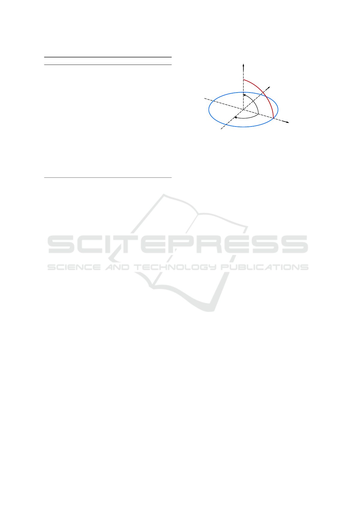
x
y
z
θ
φ
(a)
Figure 1: φ and θ as azimuth(blue) and elevation(red).
all curves to which a given point belongs are given
by all parameter values that fulfil Eq. (1). Generally,
the number of possible curves is infinite, but it can be
made finite by a discretisation of the parameter space:
each parameter p
i
is assumed to be limited to a range
of N
i
values from a finite set P
i
= {p
i1
,. .., p
iN
i
},
where the number N
i
of possible parameter values
may vary from parameter to parameter.
Each of the discrete parameter values then repre-
sents a cell in parameter space, and a point x votes
for all cells that contain parameters fulfilling Eq. (1).
To make the voting process tractable, Eq. (1) must be
rewritten as
g(x, p
1
,. .., p
k−1
) = p
k
(2)
Then all parameter cells, to which x belongs, can
be determined in a loop over all parameter values
P
1
×.. . ×P
k−1
and by computing the cell of the last
parameter through Eq. (2). The resulting algorithm is
listed as Algorithm 1.
2.2 Line Parametrisation
For the purpose of algorithmic efficiency it is advis-
able to use a parametrisation that is unique, does not
suffer from singularities and is non-redundant. Such a
parametrisation for lines in 3D that uses only four pa-
rameters (x
0
,y
0
,φ,θ) was given by Roberts (Roberts,
1988).
The direction of a line can be specified by the two
parameters φ for horizontal orientation (azimuth) and
θ for altitude (elevation) (see Fig. 1). The directional
vector
b is obtained from θ and φ through
b =
b
x
b
y
b
z
=
cosφ cosθ
sinφ cosθ
sinθ
(3)
Since two anti-parallel directional vectors describe
the same line, the vectors
b have to be confined to a
half-space for the representation to be unique. This
can be achieved by restricting the angle ranges to
VISAPP 2016 - International Conference on Computer Vision Theory and Applications
346
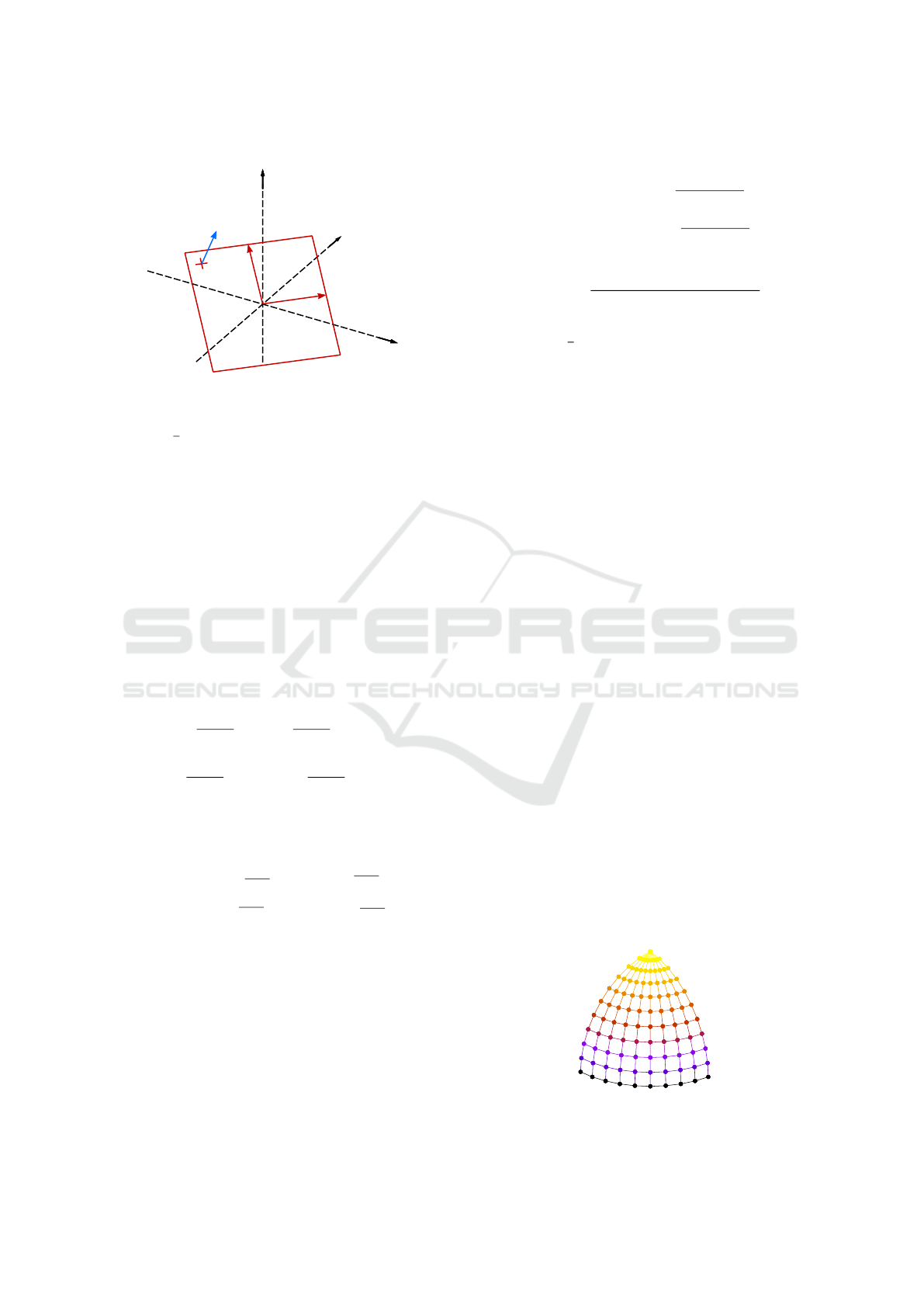
x
y
z
b
(x',y')
⃗
Figure 2: Line parametrisation by Roberts with x
0
,y
0
(red)
and the line’s directional vector
b (blue).
0 ≤ θ ≤
π
2
and −π < φ ≤ π. The remaining redun-
dancy through anti-parallel vector pairs in the (x,y)-
plane (b
z
= 0) is removed with the restrictions b
y
≥ 0
if b
z
= 0 and b
x
= 1 if b
y
= b
z
= 0.
When the position of the line is represented by
an arbitrary anchor point, this leads to three param-
eters of which one is redundant. To remove this re-
dundancy, Roberts first defines a plane which passes
through the origin and is perpendicular to the line.
The two parameters x
0
and y
0
are then defined as the
coordinates of the intersection of the line and the
plane in the plane’s own 2D coordinate frame (see
Fig 2).
From an arbitrary point p = (p
x
, p
y
, p
z
) on the
line, the parameters x
0
and y
0
are obtained with:
x
0
=
1 −
b
2
x
1 + b
z
p
x
−
b
x
b
y
1 + b
z
p
y
−b
x
p
z
(4a)
y
0
= −
b
x
b
y
1 + b
z
p
x
+
1 −
b
2
y
1 + b
z
!
p
y
−b
y
p
z
(4b)
A point p on the line can in turn be obtained with:
p = x
0
·
1 −
b
2
x
1+b
z
−
b
x
b
y
1+b
z
−b
x
+ y
0
·
−
b
x
b
y
1+b
z
1 −
b
2
y
1+b
z
−b
y
(5)
To utilise this parametrisation for a 3D Hough trans-
form, a suitable discretisation of the parameter space
has to be chosen.
2.3 Parameter Regularisation
The discretisation of θ and φ determines the orienta-
tions that can be detected by the Hough transform. A
na
¨
ıve approach is the uniform discretisation of the an-
gles θ and φ with constant step size ∆:
θ = θ
min
+ i ·∆, 0 ≤ i ≤
θ
max
−θ
min
∆
(6a)
φ = φ
min
+ j ·∆, 0 ≤ j ≤
φ
max
−φ
min
∆
(6b)
The number of resulting direction vectors is
n
uniform
=
(θ
max
−θ
min
) ·(φ
max
−φ
min
)
∆
(7)
A step size of 1
◦
, or ∆ = π/180, with −π < φ ≤ π
and 0 ≤ θ ≤
π
2
then yields a hemisphere consisting
of 32400 directional vectors. These, however, are not
equidistantly distributed on the hemisphere’s surface
(see Fig. 3). While the arc distance of adjacent vectors
on the hemisphere’s equator is ∆, it decreases as the
elevation approaches π/2.
An accumulator array, which uses these vectors
would therefore contain considerably more cells for
nearly vertical lines than for lines that are almost par-
allel to the x-axis for example. This has the effect
that the resolution for horizontal lines is much coarser
than for vertical lines. The Hough transform would
therefore be biased in favour of horizontal lines due
to their bigger cells. In other words: this parameter
space discretisation is not rotation invariant; a rota-
tion of the point cloud input to the Hough transform
would lead to different results due to the variation in
angular accuracy.
In the following, we describe two different alter-
native methods for achieving a more homogeneous
discretisation of the direction space. The aim is to
achieve an equidistant distribution of directional
vectors, so that the arc distances of neighbouring
vector end points on the hemisphere surface are
approximately constant.
Cosine-corrected Discretisation of φ. For the uni-
form discretisation (6a) & (6b) with constant angle
step size ∆, the nearest neighbour distance of direc-
tion vector end points with the same elevation θ is
d
NN
(θ) = ∆ ·cos(θ) (8)
To compensate for this effect, it is natural to make the
step-sizes for θ and φ different. When the step-size
Figure 3: Quarter hemisphere of vertices obtained by uni-
form discretisation of φ and θ.
Hough Parameter Space Regularisation for Line Detection in 3D
347
∆
θ
= ∆ is kept constant, the step-size ∆
0
φ
for φ should
increase with θ:
∆
0
φ
(θ) =
∆
θ
cos(θ)
= ∆
θ
·sec(θ) (9)
This approach, however, only provides a constant dis-
tance d
NN
(θ) = ∆
θ
in the unlikely case when ∆
0
φ
is
in integer fraction of 2π. Otherwise the arc distance
between φ
max
and φ
min
is less than ∆
0
φ
. It is thus nec-
essary to smooth out this difference and to define the
step size ∆
φ
by
∆
φ
(θ) = (φ
max
−φ
min
)
,$
φ
max
−φ
min
∆
0
φ
(θ)
%
(10)
Using ∆
θ
= ∆ and ∆
φ
(θ) for discretisation yields
an approximately equidistant direction sampling with
d
NN
(θ) ≈ ∆. The direction vectors are calculated with
θ
i
= θ
min
+ i ·∆ (11a)
φ
i j
= φ
min
+ j ·∆
φ
(θ
i
) (11b)
b
i j
=
cosφ
i j
cosθ
i
sinφ
i j
cosθ
i
sinθ
i
(11c)
where
i = 0,1, .. .,
θ
max
−θ
min
∆
θ
j = 0,1,...,
$
φ
max
−φ
min
∆
0
φ
(i ·∆ + θ
min
)
%
The number of resulting direction vectors is
n
coscorr
=
j
θ
max
−θ
min
∆
k
∑
i=0
$
φ
max
−φ
min
∆
0
φ
(i∆ + θ
min
)
%
(12)
A step size of 1
◦
(∆ = π/180) then yields 20763 in-
stead of 32400 direction vectors.
The cosine-corrected discretisation (11) indeed
reduces direction inhomogeneity and the size of
the accumulator array. But d
NN
is still only ap-
proximation constant, and direction vectors form an
irregular pattern which leads to apparently random
fluctuations of the arc distance in θ-direction. For an
approximately equidistant distribution with desirable
symmetry properties the tessellation of a Platonic
solid is preferable.
Tesselation of a Platonic Solid. In computer graph-
ics, tessellation means the process of fragmenting a
polygon into its subareas, to enable separate compu-
tation of new information and to visualise changes to
the shape of the polygon. Since graphics hardware
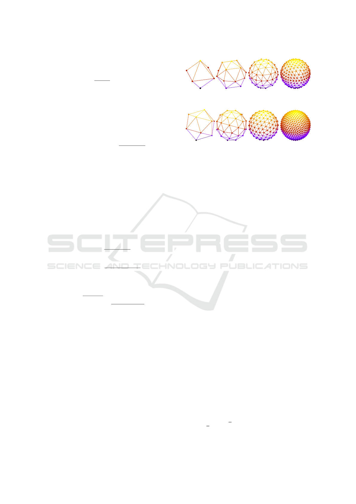
(a) (b) (c) (d)
Figure 4: Octahedron after 0,1,2,3 tessellation steps.
(a) (b) (c) (d)
Figure 5: Icosahedron after 0,1,2,3 tessellation steps.
is generally designed to process triangles, polygon
triangulation is most commonly used for tessellation
(Nvidia, 2010).
One use-case are refinement-algorithms, which
use tessellation to increase the resolution of a model
and smooth its surface. Then displacement mapping
is used, which is much more effective on polygons
with a great amount of vertices. It uses a height map
to displace the polygon’s vertices and can be used to
create detailed surface textures. Since Version 11, Mi-
crosoft’s DirectX popularly provides this technique to
increase realism in 3D graphics.
Similarly a simple polyhedron can be tessellated
repeatedly and its vertices be normalised to resemble
a unit sphere as accurately as needed. Finally, after
removing anti-parallel vectors, the resulting vertices
can be used as directional vectors for the 3D Hough
transform.
To obtain an almost uniform surface density and
a nearly equidistant distribution of the direction vec-
tors, it is advisable to use platonic solids as the start-
ing point of the tessellation because of their symmetry
properties. Each vertex of a platonic solid has the ex-
act same number of neighbouring vertices and each
edge between the vertices has the same length. A
platonic solid therefore defines an exactly equidistant
distribution of directional vectors on a sphere.
An Octahedron (see Fig. 4(a)) for example con-
sists of eight triangles, six vertices, twelve equally
long edges and is invariant under rotations by 90
◦
around any axis. Its six vertices are defined as
O =
{
(±1,0,0),(0,±1,0) ,(0, 0,±1)
}
(13)
An icosahedron (see Fig. 4(a)) consists of 20 trian-
gles, twelve vertices, 30 equally long edges and can
be defined using the golden ratio ϕ:
I =
{
(0,±1,±ϕ),(±1,±ϕ,0) ,(±ϕ, 0,±1)
}
ϕ =
1
2
1 +
√
5
(14)
VISAPP 2016 - International Conference on Computer Vision Theory and Applications
348
Each triangle can now be divided into four new ones
using polygon triangulation by inserting a new vertex
d between each pair of vertices (a,
b) of the triangle
and normalising its length:
d =
a +
b
ka +
bk
(15)
Doing so for all of the polygon triangles results in a
new vertex for each edge and three new edges for each
new vertex:
|V
0
| = |V |+ |E| (16)
|E
0
| = 4 ·|E | (17)
where V is the set of vertices, E the set of edges,
and |.| stands for the number of elements. This can
be repeated as often as necessary for the desired level
of granularity. Table 1 shows the number of unique
directions and the average nearest neighbour arc dis-
tances for different numbers of icosahedron subdivi-
sions. For six subdivisions, the arc distance approxi-
mately corresponds to 1
◦
= π/180 ≈ 0.1745.
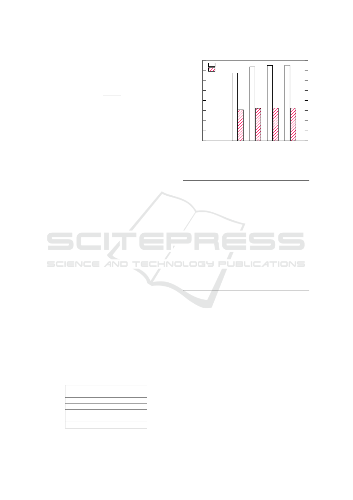
It should be noted that there is only a finite num-
ber of Platonic solids, and that vertices obtained by
subdivisions therefore cannot be exactly equidistantly
distributed. The distance variation resulting from our
method is not high, however, especially when it starts
with an icosahedron, which is the Platonic with the
largest number of vertices. The coefficient of varia-
tion c
v
= σ/µ for the length of all edges of a tessel-
lated icosahedron is much lower than that of a tessel-
lated octahedron (see Fig. 6) which implies that it is a
better approximation of an equidistant distribution.
Application to 3D Hough Transform. In Algorithm
1, there is the freedom to choose which parameters
are utilised for the predefined loops in lines 3-5, and
which remaining parameters are to be computed for
all values of the other predefined parameter values.
In our discretisation, it is much more complicate to
find the closest direction for a given direction than to
find the closest x
0
and y
0
values. Consequently, the
loop should go over the precomputed discrete direc-
tions and x
0
and y
0
are to be computed for each input
point and each direction with Eq. (4). The resulting
algorithm is listed in Algorithm 2.
Table 1: Number of directions and nearest neighbour dis-
tance d
NN
for subsequent icosahedron subdivisions.
division no. directions d
NN
1 21 0.5465
2 81 0.2794
3 321 0.1412
4 1281 0.0713
5 5121 0.0389
6 20481 0.0180
0
0.02
0.04
0.06
0.08
0.1
0.12
0.14
0.16
0 1 2 3 4
Coefficient of variation
Subdivisions
Octahedron
Icosahedron
Figure 6: Coefficient of variation c
v
= σ/µ for the length of
all edges of an Octahedron and an Icosahedron after up to 4
tessellation steps.
Algorithm 2 : Hough transform for 3D lines.
Input: point cloud X = {x
1
,. ..,x
n
},
direction vectors B = {
b
1
,. ..,
b
N
1
},
x
0
-discretisation X
0
= {x
0
1
,. ..,x
0
N
2
},
y
0
-discretisation Y
0
= {y
0
1
,. ..,y
0
N
3
}
Output: voting array A of size N
1
×N
2
×N
3
1: A(
b
i
,x
0
j
,y
0
k
) ← 0 for all
b
i
,x
0
j
,y
0
k
2: for x ∈ X do
3: for
b
i
∈ B do
4: (x
0
,y
0
) ← computed after Eq. (4)
5: (x
0
j
,y
0
k
) ← NN to (x
0
,y
0
) from X
0
×Y
0
6: A(
b
i
,x
0
j
,y
0
k
) ← A(
b
i
,x
0
j
,y
0
k
) + 1
7: end for
8: end for
9: return A
3 USE CASE: RIDGE DETECTION
To test the 3D line detection, we used airborne laser
scanning data of the city of Krefeld. The data was
scanned with an average step size of about 24cm in
the x and y direction. We combined these data with
land register data in order to extract point clouds of 20
individual buildings. We extracted candidate points
from each point based on local curvature and com-
pared the eventually detected 3D lines with the ex-
pected results. The following subsections describe the
extraction criterion for the candidate points and the
results.
3.1 Point Cloud Filtering
Our criterion for filtering ridge and edge candidates
was based on the observation that edge and ridge
Hough Parameter Space Regularisation for Line Detection in 3D
349

(a) Magnitude of highest eigenvalues (blue =
low, red = high).
(b) Filtered candidate points (green = after
global thresholding, red = after local threshold-
ing).
Figure 7: Estimated curvature (highest eigenvalue) of a sur-
face point cloud and the selected candidate points.
points should have a higher curvature than their
neighbourhood. We estimated the curvature with the
Point Cloud Library (PCL)
1
function PrincipalCur-
vaturesEstimation.
This function estimates as a first step the surface
normal for every point with an analysis of the eigen-
vectors and eigenvalues of a covariance matrix cre-
ated from the k nearest neighbours of the query point.
In our case we used k = 20, because for smaller values
of k the normals were too noisy and for higher val-
ues of k we observed rotated surface normals at the
borderline between small surfaces. Once all surface
normals have been computed, all normals from the k-
neighbourhood around a query point are projected in
the tangent plane. In the projected plane, the covari-
ance matrix of the projected lines is calculated and its
two eigenvalues are returned as the curvature estima-
tion.
We used the highest eigenvalue as a curvature es-
timation. An example can be seen in Fig. 7(a). On
these curvature values, we first performed a global
1
http://pointclouds.org/
thresholding operation by selecting all points with the
highest eigenvalue greater than 10% of the total max-
imum value and the lowest eigenvalue less than 10%
of the total maximum value (green and red points in
Fig. 7(b)). On these points, we then applied a local
threshold by removing all points with a curvature less
than the mean curvature of all k = 20 neighbors (red
points in Fig. 7(b)).
3.2 Results
For a noisy data set of 20 complete point clouds of
roofs, we have manually notated the ridges and edge
lines. This lead to the numbers of ground truth lines
listed in the column labelled n in Table 2. On the
points clouds that have been filtered as described in
section 3.1, we have applied the Hough transform
with our direction tessellation as follows: the step size
in the (x
0
,y
0
)-plane was set to 0.5, which is approx-
imately two times the NN distance in the scanning
raster, and the number of directions was set to 1281,
which corresponds to four subdivisions of an icosahe-
dron.
In the accumulator array of the Hough transform
for each roof, we selected with a non-maximum sup-
pression (Burger and Burge, 2009) the n (the number
of ground truth lines) most voted lines and counted,
how many of the ground truth lines have been de-
tected. For the non-maximum suppression, the graph
from the tesselation process was reused for neighbour
relations. Two vectors a and
b are neighbours, if there
is an edge (a,b) in the graph. For each vertex we then
defined a neighbourhood with path length l = 4 as ev-
ery vertex that can be reached with a minimum of l
edges.
The results are shown in the column labelled m
reg
in Table 2. For comparison, we have also counted
the number of correctly detected lines with the na
¨
ıve
uniform angle discretisation with approximately the
same total number of different directions (column
m
uni
in Table 2). The new method lead to an over-
all detection rate of 69/90 ≈77% of the ground truth
lines, while the na
¨
ıve discretisation only detected
54/90 = 60% of the ground truth lines. This is a clear
improvement.
A closer look at the reasons for missed ground
truth lines showed that in 11 cases a ground truth line
showed up as two similar lines detected by the Hough
transform. One example is shown in Fig. 8(a): here a
single ridge shows up as two lines due to some curva-
ture at the end. Another typical example can be seen
in Fig. 8(b): due to noise in the data, the ridge is not
represented as a line, but as a rectangle in which the
two diagonals are the longest lines and are thus de-
VISAPP 2016 - International Conference on Computer Vision Theory and Applications
350
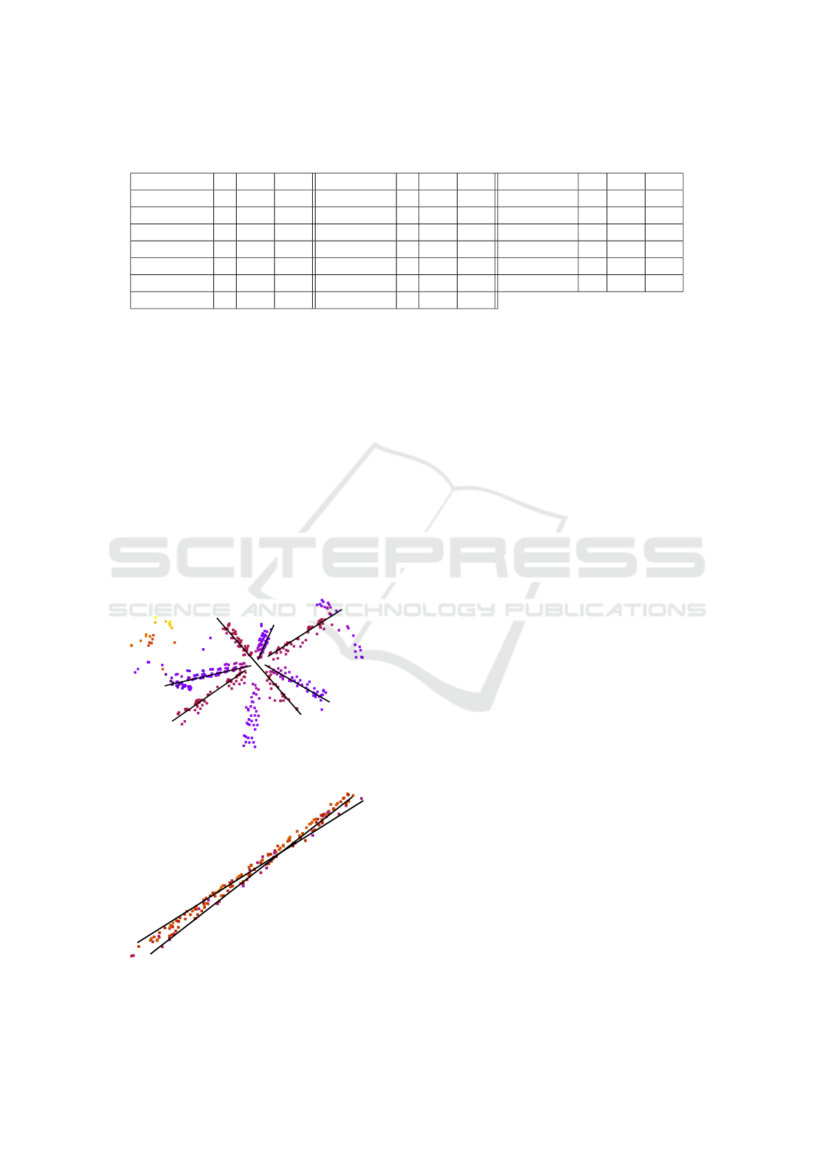
Table 2: The number of ground truth lines (n) for roofs at different locations in our dataset, and the number of detected lines
with a Hough transform with the na
¨
ıve uniform discretisation (m
uni
) and with the regularised discretisation via tessellation
(m
reg
).
location n m
uni
m
reg
location n m
uni
m
reg
location n m
uni
m
reg
Anrather 4 3 4 Glockenspitz 8 5 5 Moerser 1 1 1
Bonifatius 2 2 2 Grenz 4 2 3 Oelschlaeger 2 2 2
Buschdonk 3 2 3 Hardenberg 5 4 3 Seiden 4 3 3
Dreikoenigen 1 1 1 Huelser 6 2 5 Steckendorf 2 1 1
Evgl.Kirche 7 4 4 Ispels 9 5 7 Tannen 3 1 2
Friedr.-Ebert 7 5 7 Knein 5 1 3 Wieland 4 4 4
Gladbacher 5 2 3 Koenigs 8 4 6 total 90 54 69
tected by the Hough transform.
This means that of the 90 highest maxima in the
Hough accumulator arrays, actually 69+ 11 = 80 cor-
respond to ground truth lines. This leads to a rate
of 80/90 ≈ 89% lines among those returned by the
Hough transform that are correct.
4 CONCLUSIONS
The presented discretisation of the direction param-
eters for the Hough transform for 3D line detection
is a simple method to avoid an uneven distribution of
directions. The method is not restricted to 3D line
detection, but can be generally used for the Hough
transform when parameters in the Hough space repre-
(a) Example with five of the six lines being de-
tected. One of the ground truth lines is split up
into two different detected lines.
(b) Another example of a split line
Figure 8: Example Results of the 3D Hough Transform.
sent a direction in a 3D space, e.g. for plane detection
in 3D.
The application to ridge detection shows that the
new parameter space representation for 3D line de-
tection works quite well even on very noisy data.
The noise in our data was due to the very simple
rules for filtering candidate points that possibly be-
long to ridges. Further improvements for this specific
use case are to be expected when more sophisticated
methods are used for candidate point selection.
In this paper, we only considered discretisation
approaches that produce symmetric and regular di-
rection patterns. It would be interesting to investi-
gate how these compare to irregular patterns, e.g. ob-
tained from Fibonacci numbers (Gonz
´
alez, 2010) or
generalisations thereof (Anderson, 1996). The use
of such patterns would however make it necessary to
find a well-defined way for implementing the non-
maximum suppression. In our approach, this can
be done in a natural way, because the tesselation
algorithm produces a neighbourship graph as a by-
product.
ACKNOWLEDGEMENTS
We are grateful to the Katasteramt Krefeld for provid-
ing us with the laser scan data from Geobasisdaten der
Kommunen und des Landes NRW
c
Geobasis NRW
2014. Moreover, we would like to thank the anony-
mous reviewers for their helpful comments.
REFERENCES
Anderson, P. G. (1996). Advances in linear pixel shuffling.
In Bergum, G., Philippou, A., and Horadam, A., edi-
tors, Applications of Fibonacci Numbers, pages 1–21.
Springer, Netherlands.
Bhattacharya, P., Liu, H., Rosenfeld, A., and Thompson,
S. (2000). Hough-transform detection of lines in 3-D
space. Pattern Recognition Letters, 21(9):843–849.
Hough Parameter Space Regularisation for Line Detection in 3D
351

Burger, W. and Burge, M. (2009). Principles of Digital Im-
age Processing - Core Algorithms. Springer, London.
Gonz
´
alez, A. (2010). Measurement of areas on a sphere
using Fibonacci and latitude-longitude lattices. Math-
ematical Geosciences, 42(1):49–64.
Hough, P. V. (1962). Method and means for recognizing
complex patterns. US Patent 3,069,654.
Ishida, Y., Izuoka, H., Chinthaka, H., Premachandra, N.,
and Kato, K. (2012). A study on plane extraction from
distance images using 3D Hough transform. In Soft
Computing and Intelligent Systems (SCIS) and Inter-
national Symposium on Advanced Intelligent Systems
(ISIS), pages 812–816.
Moqiseh, A. and Nayebi, M. (2008). 3-D Hough transform
for surveillance radar target detection. In IEEE Radar
Conference RADAR ’08, pages 1–5.
Mukhopadhyay, P. and Chaudhuri, B. B. (2015). A survey
of Hough transform. Pattern Recognition, 48(3):993–
1010.
Nvidia (2010). NVIDIA GF100: World’s
fastest GPU delivering great gaming per-
formance with true geometric realism.
http://www.nvidia.com/object/IO 86775.html.
Qiu, W., Yuchi, M., Ding, M., Tessier, D., and Fenster, A.
(2013). Needle segmentation using 3D Hough trans-
form in 3D TRUS guided prostate transperineal ther-
apy. Medical physics, 40(4):042902.
Roberts, K. (1988). A new representation for a line. In
Computer Vision and Pattern Recognition CVPR’88,
pages 635–640.
Schenk, T. (2004). From point-based to feature-based aerial
triangulation. ISPRS Journal of Photogrammetry and
Remote Sensing, 58(5):315–329.
Zhou, H., Qiu, W., Ding, M., and Zhang, S. (2008). Auto-
matic needle segmentation in 3D ultrasound images
using 3D improved Hough transform. In Medical
Imaging, page 691821.
VISAPP 2016 - International Conference on Computer Vision Theory and Applications
352
