
Development of Defect Verification System of IC Lead Frame Surface
using a Ring-lighting
Yoshiharu Nakamura
1, 2
and Shuichi Enokida
1
1
Kyushu Institute of Technology, 680-4 Kawadu, Izuka, Fukuoka, Japan
2
Mitsui High Tech, Inc., 12-10-1 Komine, Yahatanishi, Kitakyusyu, Fukuoka, Japan
Keywords: Machine Vision, Defect Detection, Multiple Light Source Imaging, IC Lead Frame.
Abstract: It is especially needed for the IC lead frames used in the manufacture of semiconductors, which require both
high quality and miniaturization. To overcome above, automatic defect detection systems based on image
processing methods were proposed. Especially, this paper focuses on methods using the surface normal
direction to detect a deformation in flat parts. Since most of these methods use a fixed parameter, the risk of
missing a defect in industrial parts becomes a problem. In this paper, new defect detection method is
proposed for detecting various defect sizes and defect types. This method determines the appropriate block
size based on the median value of luminance dispersions calculated for several block sizes and learning
from a sample that detects a defect point beforehand. We used 105 samples in our experiments. Our
experimental results show our proposed method selects the superior parameters and identification of the
defect area selected is superior with learning in detecting defects of several sizes.
1 INTRODUCTION
1.1 Background of This Research
Recently, demand has grown for defect detection
processes in machine vision applications. This is
especially needed for the IC lead frames used in the
manufacture of semiconductors, which require both
high quality and miniaturization. In previous work,
we proposed a detection method that assumes the
variance in the intensity of oriented gradients in
images having defective areas is larger than that
found in normalcy areas (Nakamura et al., 2013).
Therefore, detecting defects tends to have large
variance in the local image (Aoki et al., 2013). We
performed further experiments reported in this study
by Aoki et al., for IC lead frames. However, we
confirmed that detection was difficult, when these
methods are used for verifying a deformation in flat
parts. Image processing methods by using the
surface normal direction information was proposed
to detect a deformation in flat parts (Hirose et al.,
2000; Morimoto et al., 2011; Tanaka et al., 1994).
However, most of these methods use a fixed
parameter, such as block size. When these methods
look for various defects at whole images of
industrial parts by using the same parameter, the risk
of missing a defect increases. In this paper, another
detection method is proposed for detecting various
defect sizes and defect types. To detect various
defects in industrial parts with this method, it is
necessary to change parameters according to the
size, especially, but also the kind of defect.
1.2 Purpose
In this paper, we pay attention to the defect size to
detect various defects for IC lead frames. It is
supposed that a small defect is detected by using a
defect detector of small block size, since a small
defect has a high-frequency signal. On the other
hand, it is supposed that a large defect is not
detected by using a defect detector of small block
size, since the large defect has a low-frequency
signal. It is supposed that a defect detector of the
large block size is necessary to detect the low-
frequency signal. In this paper, we propose a method
for automatically determining the appropriate block
size for the size of the defect. Fig. 1 shows the flow
of inspection processing of the proposed method.
The inspection processing comprises two phases.
In the first phase (inspection processing #1), each
Nakamura, Y. and Enokida, S.
Development of Defect Verification System of IC Lead Frame Surface using a Ring-lighting.
DOI: 10.5220/0005675801170125
In Proceedings of the 11th Joint Conference on Computer Vision, Imaging and Computer Graphics Theory and Applications (VISIGRAPP 2016) - Volume 4: VISAPP, pages 117-125
ISBN: 978-989-758-175-5
Copyright
c
2016 by SCITEPRESS – Science and Technology Publications, Lda. All rights reserved
117
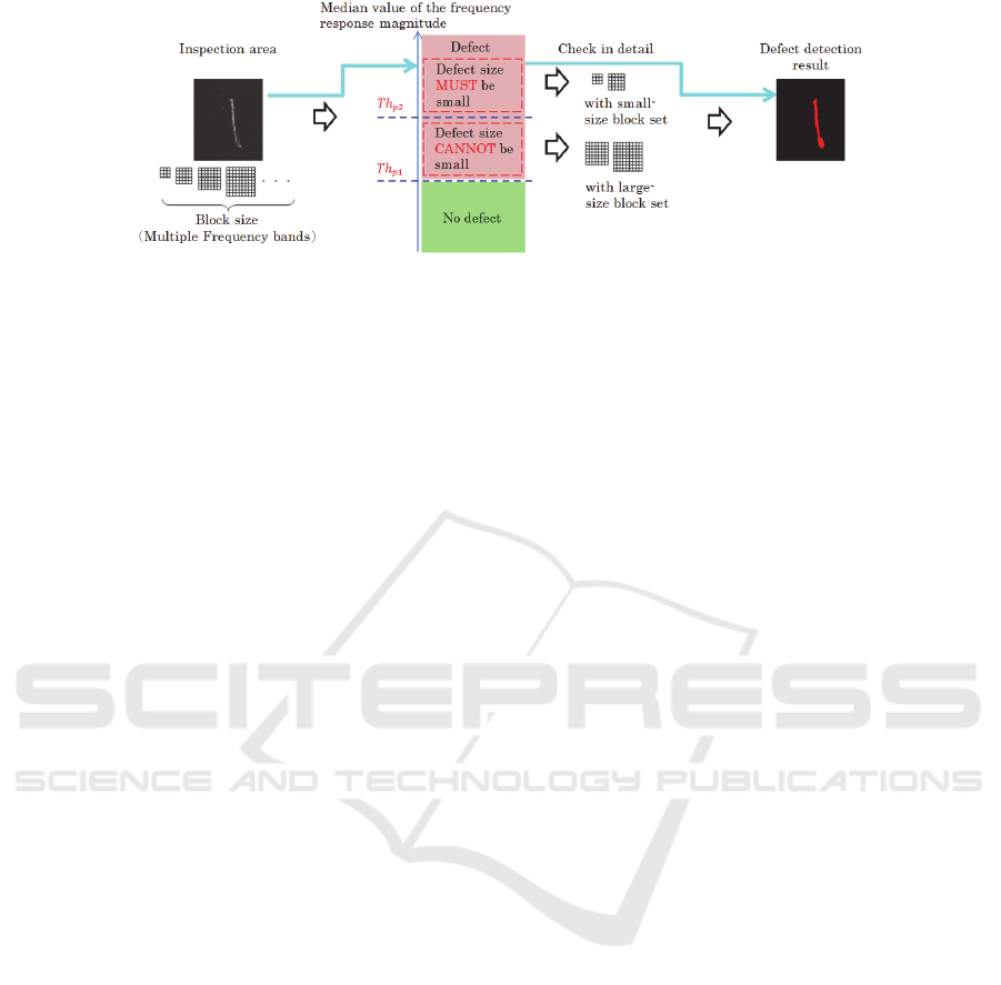
Figure 1: Flow of inspection processing of the proposed method.
inspection area is processed in all frequency bands.
Inspection processing #1 has little calculation cost.
A suspicious area detected in the first phase is
passed to the second phase (inspection processing
#2). The second phase identifies the defect position.
Compared to inspection processing #1, inspection
processing #2 has a high calculation cost. In the
second phase, it is necessary to process a small area
to identify the defect area exactly. However,
processing in a small area decreases the acquired
information about the defect. We complement the
information so that the defect can be identified even
in a small area by obtaining multiple images while
the light source direction is rotated around the
viewing direction. However, one risk is that the area
contains a lot of noise when only high-frequency
information is used. Another risk is that the number
of undetected defects increases when only low-
frequency information is used. Therefore, instead of
using a fixed block size, we use the weighted sum of
processed values in a plurality of block sizes. As a
result, a defect area is identified by reducing the
influence of the inclination of the optical system.
The block size and weight are automatically
determined by using the value in each frequency
band provided from an input image directly in
inspection processing #1 and learning from a sample
that detects a defect point beforehand. In this paper,
we use a defect detector, in which the disagreement
area of the surface normal direction and the camera
optical axis is defined as a defect, since the normal
direction of the defect area has an inclination in
comparison with that of the normalcy area. (The
normalcy area is flat in an IC lead frame.)
2 RELATION OF SURFACE
NORMAL DIRECTION AND
REFLECTED LIGHT
2.1 Reflection Models and Relation to
Surface Normal Direction
The state of light reflected from an object surface
has been represented in a variety of reflection
models. In many such reflection models, light values
are approximated by the sum of the specular and
diffuse reflection components (Mukaigawa, 2010).
Lambert models are used as a diffusion reflection
model at viewpoint of the object surface. In Eq.
(1), it is assumed that the Lambert model is
proportional to the cosine of the angle defined by the
normal direction and the direction of light source
.
max
0, ∙
(1)
where
is diffuse reflectance.
Additionally, in Eq. (2), the Phong model (Phong,
1975), which is a specular reflection model, is
approximated as the power of the cosine of angle
defined by viewing direction and specular reflection
′.
cos
(2)
where
is specular reflectance and is a parameter
representing the surface roughness.
The intensity of reflected light depends on the
surface normal direction relative to both the diffuse
reflection component (represented by the Lambert
model) and the specular reflection component
(represented by the Phong model). If the viewing
direction is parallel to the surface normal direction, the
reflected light intensity does not change when the light
source direction rotates around the viewing direction.
However, when the viewing direction is not parallel to
the surface normal direction, the reflected light intensity
VISAPP 2016 - International Conference on Computer Vision Theory and Applications
118
varies as the light source rotates around the viewing
direction. Therefore, by obtaining and analyzing multiple
images while the light source direction is rotated around
the viewing direction, it is possible to determine whether
the viewing direction is parallel to the surface normal
direction.
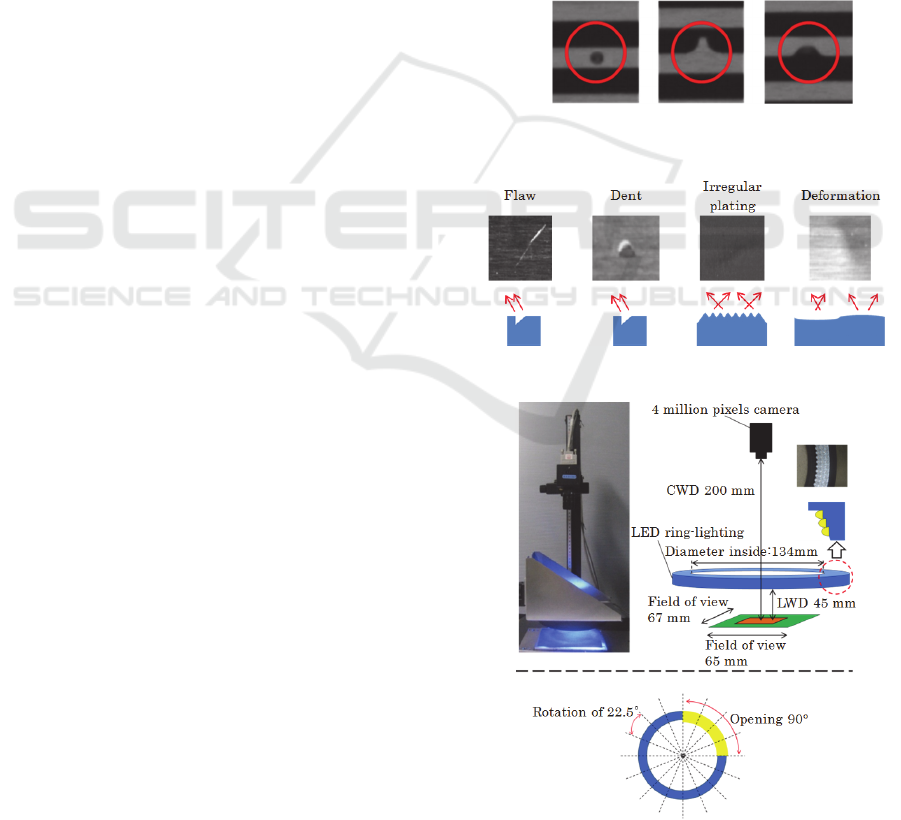
2.2 Surface Normal in the Defect Area
In previous work, we proposed a detection method
that assumed the variance in the intensity of oriented
gradients in images that include defect areas to be
larger than normalcy areas. This method targets the
example defects shown in Fig. 2 and Fig. 3. In Fig. 2,
the method effectively detects a defect in the end
face and a defect having a strong edge. However, it
could not satisfactorily detect a defect not having a
strong edge and a defect shaped as a rectilinear
figure in a flat area, as shown in Fig. 3. Therefore,
for the defect shown in Fig. 3, we use a defect
detector in which the disagreement area of the
surface normal direction and the camera optical axis
is defined as a defect, since more inclination is
found in the surface normal direction than in the
normalcy area in the defect area due to the normalcy
area being flat in IC lead frames. The inclinations of
the surface normal directions in the defect area are
shown in Fig. 3.
3 INSPECTION METHOD
3.1 Inspection Equipment
Fig. 4 shows the experimental environment used to
acquire images. We rotated a light emitting diode
(LED) ring-lighting, which opening 90° in 22.5°
increments in order to acquire 16 images while
varying the direction of incident illumination.
3.2 Agreement or Disagreement of
Normal Direction and Camera
Optical Axis
In this paper, defects are detected by using the
variance calculated by using multiple images
acquired by varying the light source direction. If the
viewing direction is parallel to the surface normal
direction, the reflected light intensity does not
change when the light source direction rotates
around the viewing direction. However, when the
viewing direction is not parallel to the surface
normal direction, the reflected light intensity varies
as the light source rotates around the viewing
direction.
Therefore, by obtaining and analyzing multiple
images while the light source direction is rotated
around the viewing direction, we are able to
determine whether a defect is detected. Originally, it
was expected that detection of a defect was possible,
when the shape of the defect was estimated by using
the photometric stereo method (Woodham, 1980)
with multiple light sources. However, the estimate of
a detailed shape had a high calculation cost. In
addition, since the information that we want to get is
whether a defect exists, detailed shape information is
not required. Therefore, we decided to apply the
proposed method, which identifies only the
reflection intensity of light changes by the
inclination of the normal direction.
Figure 2: Defect with variance in the intensity of oriented
gradients.
Figure 3: Defects and surface normal directions.
Figure 4: Imaging environment.
Development of Defect Verification System of IC Lead Frame Surface using a Ring-lighting
119

3.3 Inspection Processing
As mentioned above, the inspection processing
comprises two phases. The first phase determines
whether a defect exists for each inspection area
(inspection processing #1). The second phase
identifies a defect area for an area determined to
include a defect in inspection processing #1
(inspection processing #2).
3.3.1 Inspection Processing #1: Determining
Whether a Defect Exists
The first phase determines whether a defect exists
for each inspection area. The variance value
is
used for the determination.
determines a defect by
identifying the areas of brightness change by the
inclination of the normal direction of the defect in a
large area.
can determine a defect if a defect
having a different brightness is in the peripheral area,
because the variance values of the block are
increased.
is calculated by using the maximum of
the measured variance values. These values are
calculated for (=1, 2・・・) images acquired
from several light source directions (Fig. 5). By
using the maximum value, it is possible to use a light
source direction in which the defect has the largest
brightness difference.
,
1
,
(3)
,
max
∈
,
where
is block size,
is the mean in the block.
A raster scan of the inspection area is performed
and
is computed for all pixels using Eq. (3).
To detect defects having various frequency bands,
various block sizes are prepared. The processing
calculates the maximum value of
for each
different block size, and then obtains the median
value from the maximum value for each different
block size (median
). The proposed method
compares median
with the threshold
.
median
median
max
,
median
(4)
where is the position the inspection area.
By using the median value from the maximum
value for each different block size, if a defect exists,
the
value is larger for that block size. Then, the
existence of a defect can be determined robustly,
while reducing the influence of noise in a particular
block size.
3.3.2 Inspection Processing #2: Defect Area
Is Identified
In the second phase, a defect area is identified for an
area already determined to include a defect in
inspection processing #1. It is necessary to process a
small area to identify a defect area exactly. If the
block size is small,
values used in inspection
processing #1 cannot obtain sufficient variance
values for the defect, since
values are calculated
for each light source direction. Therefore,
is used
to determine whether the normal direction at the
point (or small region) of interest is parallel to the
camera's optical axis.
is calculated in the same
block by using multiple images, which are acquired
by varying the ( = 1, 2・・・) direction of the
light source (Fig. 6).
,
1
・
,,
(5)
where
is block size,
is the mean in the
block.
A raster scan of the inspection area is performed and
is then computed for all pixels by Eq. (5). This
value of
is used to determine whether the normal
direction at the point (or small region) of interest is
parallel to the camera’s optical axis. However, this
assessment alone is inadequate when the stage has
only a slight tilt with respect to the optical axis (Fig.
7) and has a lot of noise. Therefore,
must
overcome this problem. Because
is capable of
discriminating between the flat and curved areas at a
(large) surface area of interest, it overcomes the
problem that results when the stage is tilted with
respect to the optical axis. Finally, the weighted sum
of
and
is utilized to detect defects.
and
are normalized at each maximum. Defect detection
is then performed by using α, which determines the
weight of the
value, the
value, and , which
determines the detection level.
Figure 5:
calculation method.
VISAPP 2016 - International Conference on Computer Vision Theory and Applications
120
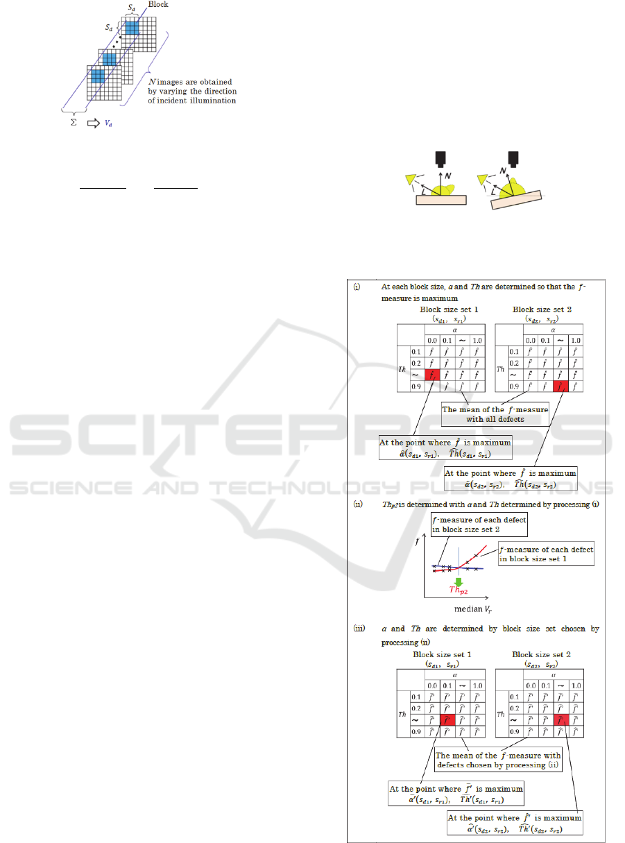
Figure 6:
calculation method.
1
,
max
,
max
(6)
The block sizes used for
and
that make s
> s
because
is calculated in a small region and
is
calculated in a large region.
In the inspection, the determination of each
parameter (block size set ( s
, s
), α , ) is
important. Each parameter is automatically
determined by learning with some samples
containing a defect. The -measure, which is the
harmonic average of the ratio of the detected area to
the total correct answer area and ratio of the correct
answer area to the total detected area, is used as a
learning indicator. (By using the harmonic average,
if the one is remarkably lower than the other, the
influence of the one is suppressed.) The
determination of the block size set uses the median
value calculated for each inspection area in
inspection processing #1. If the median
value is
large, because it is presumed that a high-frequency
defect exists, it is necessary to find the exact defect
area by using a small block size set. If median
value is small, because it is presumed that a low-
frequency defect exists, it is necessary to find the
defect in a large area by using a large block size set.
The flow of learning is shown below (Fig. 8).
(i) First, in order to determine α and for each
block size set, the defect area is detected and
the -measure is calculated by Eq. (6) and
using the learning defect samples. The average
of the -measure of all defect samples is
calculated (
-measure), and α and are
determined by the biggest
-measure for each
block size set.
(ii) The block size set is determined for each defect
sample.
is assigned to separate each
defect sample so that the -measure is bigger.
Fig. 8 (ii) are plots with the median
of each
defect sample and the -measure with α and
determined in (i). The block size set is
determined by whether median
of each
defect sample is larger or smaller than
.
(iii) The average of the -measure (′
-measure) is
calculated at each block size set determined for
each defect sample, and the final α and are
determined by the biggest ′
-measure for each
block size set.
It is necessary to repeat (ii) and (iii) to obtain the
necessary precision. An area is inspected by using
each determined parameter.
Figure 7: Proper and improper optical system alignments.
Left: Ideal condition, Right: Lead frame inclining in
relation to the camera.
Figure 8: Self-adjusting parameters.
Development of Defect Verification System of IC Lead Frame Surface using a Ring-lighting
121
4 EXPERIMENTS AND RESULTS
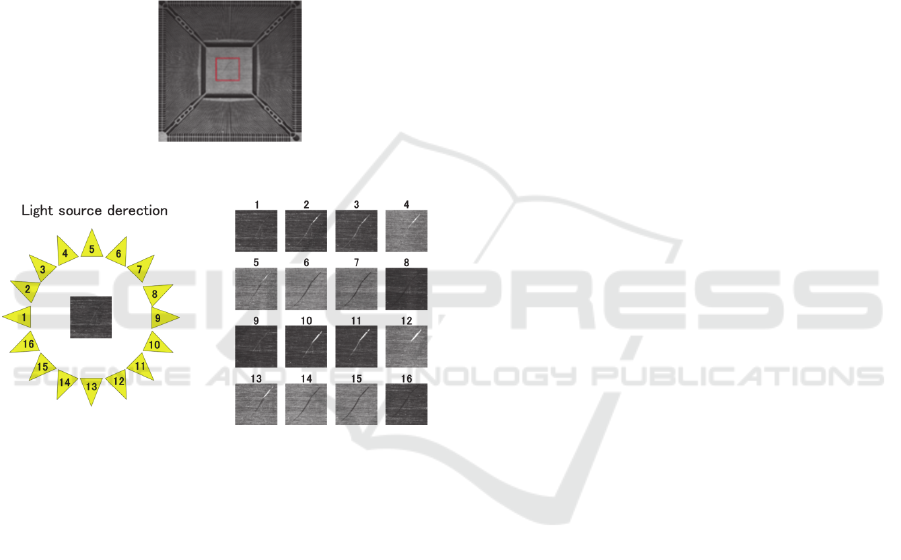
4.1 Test Sample and Images
We used 105 samples in our experiments (Defect-
free samples: 41, Flaw: 16, Dent: 16, Irregular
plating: 16, Deformation: 16). Fig. 9 shows an
example of an IC lead frame that has a flaw in the
center. Multiple images of each defect were acquired
from the 16 light source directions (Fig. 10). In our
experiment, each sample was processed by
inspection processing #1 and inspection processing
#2.
Figure 9: IC lead frame with a flaw.
Figure 10: Multiple light source imaging.
4.2 Results of Determination of the
Parameters by the Learning
The results of defect detection based on the
parameters of block sizes s
and s
, weight α
,
and
threshold , which are automatically determined by
learning, are shown in Figs. 11–13. In this
experiment, because it was a fundamental
experiment to identify the performance of the
proposed method, a block size set was either a large
set or a small set (
,
= (3, 9) or
,
= (5,
25)), and the learning was 1 loop (s
and s
were
appropriately examined in the experiment). The
results of these three figures are shown from top to
bottom in the following order: original image—
correct answer image—result of the parameter when
the
-measure is the largest in the small block size
set without learning—result of the parameter when
the
-measure is the largest in the large block size
set without learning—result of the parameter that is
automatically determined by the proposed method.
Fig. 11 shows examples of the results determined
to be in the small block size set by the proposed
method. Fig. 12 shows examples of the results
determined to be in the large block size set by the
proposed method. By comparing the results of the
proposed method with the results of each block size
set without learning, it was confirmed in Figs. 11
and 12 that identification of the defect area selected
was superior with learning. This result shows that
the method selected the superior block size set and α
and were changed to more appropriate values.
However, in some cases the method failed to select
the superior block size set. Examples that failed in
the selection of the block size sets are shown in Fig.
13. These were selected to be in the block size set
“large” by the proposed method. However, the block
size set “small” was accurate for identification of the
defect area, according to the images without learning.
It is possible that learning became specialized for a
learning sample. Therefore, it is necessary to
examine a learning method not specialized for a
defect sample as a future problem.
4.3 Results of Inspection Processing #1
4.3.1 Experimental Condition
For all 105 samples, inspection process #1
determined whether a defect existed for each
inspection area. The variance for detecting a defect
at each inspection area was
. The following block
sizes were examined in the experiment:
= 9, 17, 25,
33, 41, and 49. Median
was calculated for each
defect sample. Then, median
was compared to the
threshold to determine whether it was a defect. A
brightness difference occurs with each image
acquired by varying the light source direction, as
shown in Fig. 14 for processing a hairline on a
surface. It was confirmed that the separation of the
defect was difficult in a prior experiment. Therefore,
we used only a parallel light source direction for the
hairline (light source directions are #1, 2, 8, 9, 10,
and 16 in Fig. 10).
4.3.2 Results of Experiment and Discussion
In the defect inspection experiment, we analyzed a
characteristic of the proposed method with two
thresholds. The first is the threshold when the recall
ratio of the defect is 100% and false positives (false
detection) are minimum.
VISAPP 2016 - International Conference on Computer Vision Theory and Applications
122
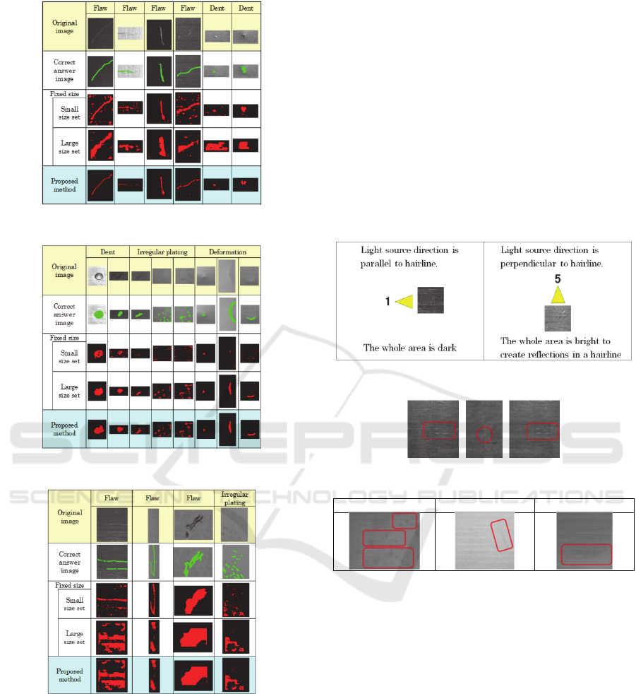
Figure 11: Examples of “the block size set is small”.
Figure 12: Examples of “the block size set is large”.
Figure 13: Examples of failed selection.
The second is the threshold when the precision ratio
is 100% and false negatives (overlooking) are
minimum. With the first threshold, 6 samples were
detected as a defect among 41 defect-free samples.
The examples of false detection are shown in Fig.
15. According to Fig. 15, defects were detected
excessively for the sensitive threshold, since
multiple points with brightness differences exist. It
is thought that these should be reexamined rather
than overlooked, since these are difficult to classify
as a defect of a flaw or irregular plating. With the
second threshold, 3 samples were overlooked as a
defect among 64 defect samples. The examples of
overlooked samples are shown in Fig. 16. According
to Fig. 16, the defect of a small brightness difference
was overlooked. In inspection processing #1, it is
thought that the excessive threshold should be used,
because it is necessary to prevent overlooking
defects, even if some defect-free products are
detected as defects. Therefore, the first threshold
should be used. The results show that the proposed
method is effective for the detection of defects of
various types and sizes.
Figure 14: Hairline on surface and light source direction.
Figure 15: Examples of error detection images.
Irregular plating Irregular plating Deformation
Figure 16: Examples of undetected images.
4.4 Results of Inspection Processing #2
4.4.1 Experimental Condition
In this experiment, defect areas are identified for 64
defect samples. These 64 samples are distributed
into 4 sets of 16 samples, and 3 sets are used for
learning to determine the parameter, and we evaluate
the detection with the one remaining set. The data
set is replaced and new learning and data sets are
created, then assessed 4 times. As mentioned in
Section 3, a brightness difference occurs with each
image acquired by varying the light source direction,
since the processing was for a hairlined surface.
Therefore, we used each image by flattening the
histogram.
Development of Defect Verification System of IC Lead Frame Surface using a Ring-lighting
123

4.4.2 Results of Experiment and Discussion
As the results of 4 iterations of evaluation by
replacing the data set, the rate of success of
identifying a defect area was 84.4%. Examples of
successful specific defect areas are shown in Fig. 17.
Examples of failure detections are shown in Fig. 18.
In this experiment, when identification of a
defect area was investigated for each kind of defect,
it was confirmed that a deformation could be
identified in all samples. The proposed method
identified all cases of a deformation with a large
normal change, by judging whether the camera
optical axis was parallel to the normal direction.
However, identification failed in the case of
some of the other types of defects.
For the dent and the irregular plating, a tendency
of failure of common defect identification was
confirmed. A large area other than the defect area
was detected. The dent had a rapid change in the
normal direction, however, the defect area was too
small. Irregular plating had too small a brightness as
compared with the peripheral area. Therefore,
separation of the intensity variation of the
background texture was difficult when such defect
areas were identified. To further improve the
performance, a way to establish a parameter apart
from a parameter of deformation with a large normal
change must be considered. We will investigate the
parameters of the method in the future.
For the flaw, both of the areas were detected
excessively and areas with a defect were overlooked.
In the proposed method, we conclude that it is
difficult to classify a surface hairline, such as a
linear defect (flaw). For detecting a defect such as a
flaw, we consider it necessary to improve the
precision in combination with image processing
techniques shown in previous work (Nakamura et al.,
2013).
Figure 17: Examples of successful detection images.
Figure 18: Examples of error detection images.
5 CONCLUSIONS
In this paper, we propose a method for automatically
determining the appropriate block size for the size of
defects to detect defects of various sizes that occur
in the surface of IC lead frames. We showed that it
was possible to detect defects that were previously
difficult to identify by conventional methods. We
used the weighted sum of two values. The one is that
identify the areas of changing brightness by the
inclination of the normal direction of the defect in a
large area. The other is that determines whether the
normal direction at a point of interest is parallel to
the camera’s optical axis by using the inclination of
the normal direction on the surface of the defect
area. As future work, it is necessary to examine a
learning method that is not specialized for a defect
sample. We are also planning to develop a system
that can detect whole parts by using the image
processing method that detects the end face of a part
together with the proposed method that detects the
flat area of a part.
REFERENCES
Nakamura, Y., Masuzoe, M., & Enokida, S., 2013. Study
of Defect Verification based on Histogram of Oriented
Gradients in Local Area. The Institute of Image
Electronics Engineers of Japan, 264th study meeting.
Aoki, K., Funahashi, T., Koshimizu, H., & Miwata, Y.,
2013. “KIZUKI” Algorithm Inspired by Peripheral
Vision and Involuntary Eye Movement. Journal of the
Japan Society for Precision Engineering, Vol. 79, No.
11, 1045-1049.
Hirose, O., Ishii, A., Hata, S., & Washizaki, I., 2000.
Detection of Small Convex and Concave Defects on
Optical Films by Patterned Illumination. Journal of
the Japan Society of Precision Engineering, Vol. 66,
No. 7, 1098-1102.
Morimoto, Y., Fujigaki, M., & Masaya, A., 2011.
VISAPP 2016 - International Conference on Computer Vision Theory and Applications
124

Displacement and Strain Distribution Measurement by
Sampling Moire Method. Journal of the Vacuum
Society of Japan, Vol. 54, No. 1, 32-38.
Tanaka, K., Shinbara, Y., Ikeda, H., Yamada N., Kiba, H.,
& Sasanishi. K., 1994. Automated Inspection Method
for Painted Surfaces. Transactions of the Japan
Society of Mechanical Engineers, C 60(577), 3201-
3208.
Mukaigawa, Y., 2010. Measurement and Modeling of
Reflection and Scattering. IPSJ SIG Technical Report,
Vol. 2010-CVIM-172, No. 34.
Phong. B. T., 1975. Illumination for Computer Generated
Pictures. Proc. SIGGRAPH’75, 311-317.
Woodham, R. J., 1980. Photometric Method for
Determining Sur-Face Orientations from Multiple
Images. Optical Eng., 19, 139-144.
Development of Defect Verification System of IC Lead Frame Surface using a Ring-lighting
125
