Benchmarking RGB-D Segmentation: Toy Dataset of Complex Crowded

Scenes

Aleksi Ikkala, Joni Pajarinen and Ville Kyrki

Department of Electrical Engineering and Automation, Aalto University, Espoo, Finland

Keywords:

Object Segmentation, RGB-D Segmentation, Benchmarking, Dataset, Complex Objects, Real World Objects.

Abstract:

In this paper we present a new RGB-D dataset

captured with the Kinect sensor. The dataset is composed

of typical children’s toys and contains a total of 449 RGB-D images alongside with their annotated ground

truth images. Compared to existing RBG-D object segmentation datasets, the objects in our proposed dataset

have more complex shapes and less texture. The images are also crowded and thus highly occluded. Three

state-of-the-art segmentation methods are benchmarked using the dataset. These methods attack the problem

of object segmentation from different starting points, providing a comprehensive view on the properties of

the proposed dataset as well as the state-of-the-art performance. The results are mostly satisfactory but there

remains plenty of room for improvement. This novel dataset thus poses the next challenge in the area of

RGB-D object segmentation.

Available at http://robosvn.org.aalto.ﬁ/software-and-data.

1 INTRODUCTION

Object segmentation from visual sensor data is one

of the most important tasks in computer vision. Seg-

mentation of RGB-D scenes is especially crucial for

robots handling unknown objects, an application area

of special interest to us. As more efﬁcient segmen-

tation methods have become available, the detection

of simple objects is readily accomplished. These ob-

jects may be, for instance, cereal boxes, coke cans,

or bowls, which embody somewhat elementary ge-

ometrical shapes and easily distinguishable textures.

Benchmarking segmentation algorithms is important

to understand the state-of-the-art performance as well

as open problems, and many useful datasets, includ-

ing the Object Segmentation Database (Richtsfeld

et al., 2012), RGB-D Object Dataset (Lai et al., 2011),

BigBIRD (Singh et al., 2014), and the Willow Garage

Dataset

, are available, containing hundreds of such

RGB-D images.

Many of the objects we encounter in our daily

lives are, however, far more complex in terms of their

shape and texture. A good example of such an object

is an ordinary child’s toy, which may or may not re-

semble any simple geometrical shape. Furthermore,

Available at http://www.acin.tuwien.ac.at/forschung/

v4r/mitarbeiterprojekte/willow/.

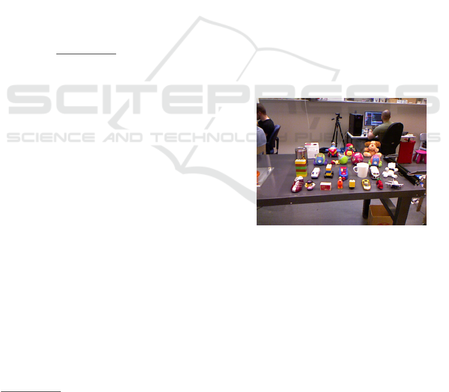
Figure 1: Toys used in the toy-dataset.

the toy may be uni- or multicolored. Our proposed

toy-dataset contains objects like this, often in crowded

scenes and occluded positions, and poses the next

challenge in the area of object segmentation towards

general purpose understanding of complex domestic

environments. The dataset consists of 449 RGB-D

images with human-annotated ground truth.

Three state-of-the-art RGB-D segmentation meth-

ods are benchmarked using the dataset, in order to

explore the dataset’s properties as well as to assess

state-of-the-art capabilities in these kind of scenes.

The methods are provided by the Vision for Robotics

group (V4R) (Richtsfeld et al., 2012), the Image

Component Library (ICL) (Uckermann et al., 2013),

Ikkala, A., Pajarinen, J. and Kyrki, V.

Benchmarking RGB-D Segmentation: Toy Dataset of Complex Crowded Scenes.

DOI: 10.5220/0005675501070116

In Proceedings of the 11th Joint Conference on Computer Vision, Imaging and Computer Graphics Theory and Applications (VISIGRAPP 2016) - Volume 4: VISAPP, pages 107-116

ISBN: 978-989-758-175-5

107

and the Locally Convex Connected Patches (LCCP)

segmenter (Stein et al., 2014) available in Point Cloud

Library (PCL, (Rusu and Cousins, 2011)).

Section 2 puts our contribution in context by re-

viewing existing RGB-D datasets. Section 3 describes

in detail our proposed dataset and some of its char-

acteristics. In Section 4 we discuss brieﬂy how the

three state-of-the-art segmentation methods function,

and also present the experiments and results on the

toy-dataset. In Section 5 the results are analyzed, and

Section 6 states the conclusion.

2 RELATED WORK

Several datasets exist for benchmarking segmentation

algorithms. Most of these previous datasets have con-

centrated on relatively simple objects comprised of

primitive shapes, such as cuboid and spherical shapes,

cylinders and combinations of these.

Among the most popular RGB-D datasets are the

Willow Garage dataset and the OSD (Richtsfeld et al.,

2012), both created with a Kinect v1. The Willow

Garage dataset contains 176 images of household ob-

jects with a little or no occlusion, as well as pixel-

based ground truth annotation. The OSD consists

of similar type of household objects as the Willow

Garage dataset. The OSD contains a total of 111 im-

ages of stacked and occluding objects on a table along

with their pixel-based annotated ground truth images.

Both of the aforementioned datasets include roughly

20-30 objects with relatively simple cylindrical and

cuboidal shapes and diverse texture.

Two popular datasets, the RGB-D Object Dataset

(Lai et al., 2011) and BigBIRD (Singh et al., 2014),

utilize a turntable to obtain RGB-D images of com-

mon household items. In addition, both datasets have

been recorded using two cameras, an RGB-D camera

and a higher resolution RGB camera. The data is gen-

erated by capturing multiple synchronized images of

an object while it spins on the turntable for one revo-

lution.

The RGB-D Object Dataset is one of the most ex-

tensive RGB-D datasets available. It comprises of 300

common household objects and 22 annotated video

sequences of natural scenes. These natural scenes in-

clude common indoor environments, such as ofﬁce

workspaces and kitchen areas, as well as objects from

the dataset. The dataset was recorded with a proto-

type RGB-D camera manufactured by PrimeSense to-

gether with a higher resolution Point Grey Research

Grasshopper RGB camera. Each object was recorded

with the cameras mounted on three different heights

to obtain views from the objects from different angles.

The BigBIRD dataset provides high quality RGB-

D images along with pose information, segmenta-

tion masks and reconstructed meshes for each ob-

ject. Each one of the dataset’s 125 objects has been

recorded using PrimeSense Carmine 1.08 depth sen-

sors and high resolution Canon Rebel T3 cameras.

The objects in the RGB-D Object Dataset and Big-

BIRD dataset are, however, mainly similar to the ge-

ometrically simple objects in the Willow Garage and

OSD datasets. In addition, apart from the video se-

quences of the RGB-D Object Dataset, the images do

not contain occlusion.

The datasets provided by Hinterstoisser et al.

(Hinterstoisser et al., 2012) and Mian et al. (Mian

et al., 2006; Mian et al., 2010) contain more compli-

cated objects than the previously mentioned datasets.

The dataset of Hinterstoisser et al. consists of 15

different texture-less objects on a heavily cluttered

background and with some occlusion. The dataset

includes video sequences of the scenes, and a total

of 18,000 Kinect v1 images along with ground truth

poses for the objects. As this dataset is more aimed

for object recognition and pose estimation, it does not

include pixel-based annotation of the objects. The

dataset proposed by Mian et al. comprises of ﬁve

complicated toy-like objects with occlusion and clut-

ter. The 50 depth-only images have been created us-

ing a Minolta Vivid 910 scanner to get a 2.5D view of

the scene. The dataset includes also pose information

for the objects and pixel-based annotated ground truth

images.

As opposed to the completely textureless and uni-

colored objects in the dataset by Hinterstoisser et al.,

the objects in our dataset retain some texture and

many are also multicolored. Also, the dataset by Mian

et al. contains only depth data, and is considerably

smaller than our proposed dataset.

Multiple RGB-D datasets have been gathered

from the real world as well. For instance, the video

sequences of the RGB-D Object Dataset, Cornell-

RGBD-Dataset (Anand et al., 2011; Koppula et al.,

2011) and NYU Dataset v1 (Silberman and Fergus,

2011) and v2 (Silberman et al., 2012) contain al-

together hundreds of indoor scene video sequences,

where the three latter datasets were captured with

Kinect v1. These sequences are recorded in typi-

cal home and ofﬁce scenes, such as bedrooms, liv-

ing rooms, kitchens and ofﬁce spaces. The images

are highly cluttered, and all the scenes in Cornell-

RGBD-Dataset are labeled, and a subset of the im-

ages in NYU Datasets contain labeled ground truths.

However, these scenes involve generally larger ob-

jects, such as tables, chairs, desks and sofas, which

are not the kind of objects a lightweight robot typi-

VISAPP 2016 - International Conference on Computer Vision Theory and Applications

108

cally manipulates.

3 TOY-DATASET

Our proposed dataset is comprised of complex objects

and annotated ground truth images. The dataset con-

tains objects which one would expect a robot to ma-

nipulate, that is, small, lightweight, and complex ob-

jects that one encounters in day-to-day life.

The objects that were chosen into the dataset rep-

resented typical children’s toys. In other words, the

objects were generally multicolored, had a little or no

texture and were of varied shapes. The objects were

placed randomly on the tabletop; the only criteria was

that they are close to one another, so that a consider-

able amount of occlusion is present.

First, we describe in detail how the dataset was

acquired and how the ground truth images were anno-

tated. Secondly, we contrast the proposed dataset to

OSD by comparing the F-scores of V4R’s features on

toy-dataset to the F-scores on OSD, and use them to

describe some of the characteristics of the toy-dataset

compared to OSD.

3.1 Set-up

The dataset consists of 449 RGB-D images and cor-

responding annotated ground truth images. The dis-

tance between the Kinect and the closer edge of the

table, the further edge of the table, and the center of

the table are roughly 85, 150, and 115 centimeters,

respectively. There are 24 toys in the dataset in to-

tal, and, compared to the toys in the OSD, many of

the toys are smaller in size. Most toys are multicol-

ored and contain only minute texture. The number of

toys per image varies according to Table 1. There are

plenty of images with only a few toys to make sure

model-based methods, such as V4R’s segmenter, are

able to learn the correct relations of an object and be-

tween objects. The complete set of toys used in this

dataset can be seen in Figure 1.

Table 1: The number of toys per image varies according to

the index number of the images. The column on the left in-

dicates the index number of an image, while the column on

the right indicates the number of toys in the corresponding

image.

# image # toys

0 – 228 2 – 4

229 – 338 6 – 7

339 – 448 14 – 18

The ground truth images were annotated manu-

ally. The pixels belonging to each object were col-

ored with a different grayscale value, while the back-

ground has a value of zero. The pixels are not anno-

tated impeccably, since the edges of objects are not

strictly one pixel wide but instead can span several

pixels. Additionally, the edges of the objects are not

always visible, because of, for example, the lighting

of the image. Moreover, since the objects are highly

occluded in most images, in some occasions it is ex-

tremely difﬁcult to distinguish which aggregation of

pixels belongs to which object.

Furthermore, we ﬁltered the point clouds such that

only the table and the objects remained. These ﬁl-

tered images are then used in our experiments, as ex-

plained in Section 4. The ﬁltering is easy to imple-

ment since the planar tabletop can be easily and ro-

bustly detected. The toy-dataset contains both the ﬁl-

tered and the original RGB-D images.

3.2 Characteristics

The discrimination capability of a feature can be eval-

uated by computing an F-score for the feature (Chen

and Lin, 2006). F-score measures the discrimination

of two sets of real numbers and it is often used for fea-

ture selection. A higher F-score indicates that a fea-

ture is more likely to be discriminative, but unfortu-

nately it does not reveal mutual information amongst

several features. Nevertheless, the F-score measure

is widely used in the machine learning literature due

to its simplicity. The F-score is deﬁned in Equation

(1): r

, k = 1, . . . , m, are the training vectors, n

and

−

are the number of positive and negative instances,

respectively. Further, ¯r

, ¯r

(+)

and ¯r

(−)

are the aver-

age of the i

feature of the whole, positive and neg-

ative datasets, respectively, and r

(+)

k,i

and r

(−)

k,i

are the

features of the k

positive and negative instances,

respectively.

We exploit the F-score and V4R’s features (as pre-

sented in (Richtsfeld et al., 2014)) in order to explore

the characteristics of our dataset. These F-scores are

then compared to those of OSD, as given in (Richts-

feld et al., 2014). OSD is also a suitable comparison

dataset as it is similar to our dataset in the sense of

how the images are obtained and how the objects are

placed. The datasets differ critically in the objects that

are used, the objects in toy-dataset having more com-

plex shapes and less texture; also, the images in our

dataset have more occlusion.

The comprehensive set of features chosen by V4R

contains commonly used features in computer vi-

sion. They measure relevant aspects of objects in

the dataset, such as texture and color information.

Benchmarking RGB-D Segmentation: Toy Dataset of Complex Crowded Scenes

109

F(i) =



¯r

(+)

− ¯r





¯r

(−)

− ¯r



−1

∑

k=1



(+)

k,i

− ¯r

(+)



−

−1

∑

−

k=1



(−)

k,i

− ¯r

(−)



(1)

This makes the V4R features suitable for compar-

ing the characteristics of these two datasets. This

same analysis could have been carried out using any

other dataset, since the procedure is easy to imple-

ment. Furthermore, the analysis is beneﬁcial as it

gives quantitative results.

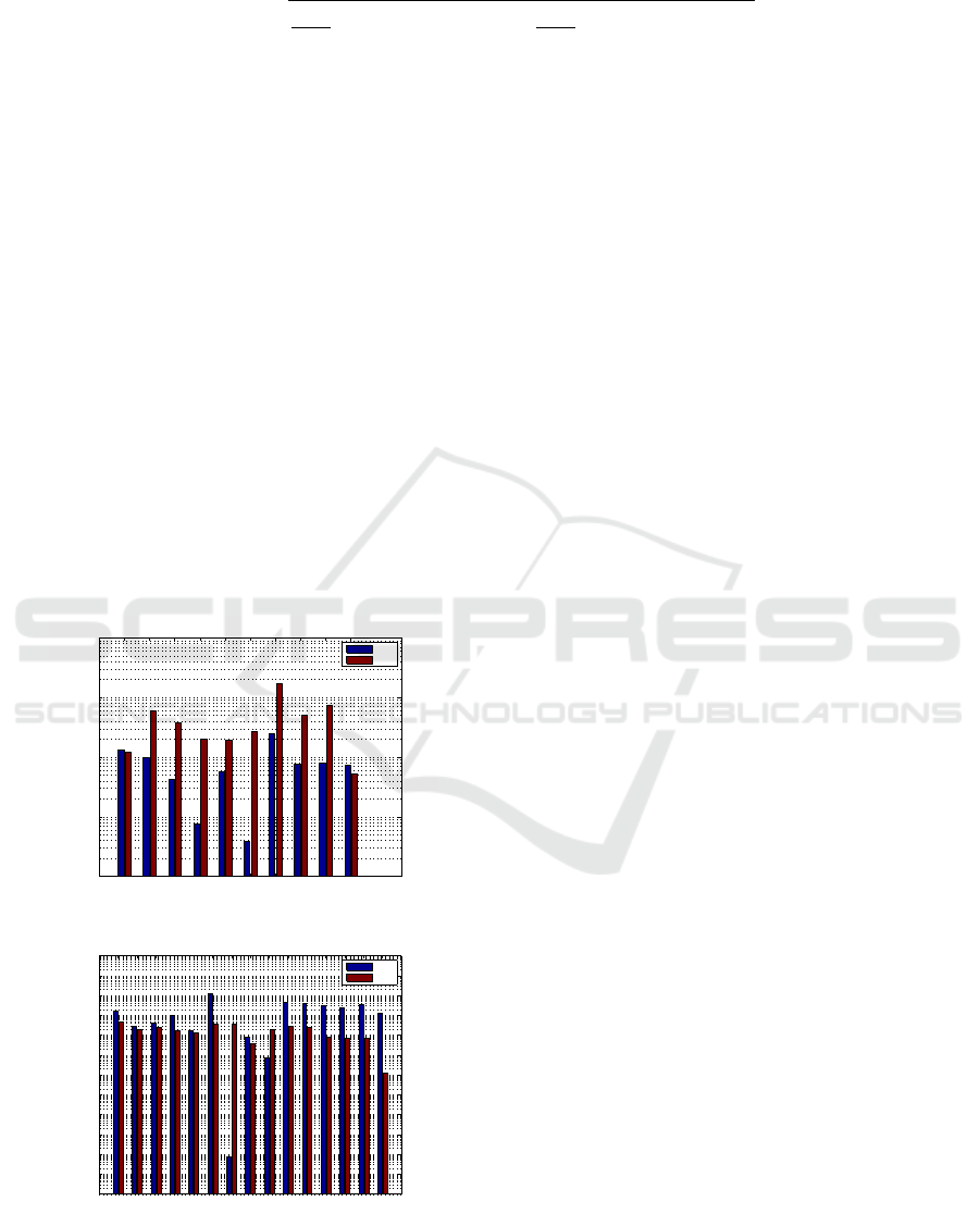
Figure 2 displays the F-scores for structural and

assembly level features for both the OSD and toy-

dataset. Structural features capture information such

as texture and color while assembly level features

capture higher level information such as distance be-

tween presegmented patches and angle between sur-

face normals of the patches. These are explained in

more detail in Section 4.1. The ﬁgure shows that

structural level features are generally smaller in the

toy-dataset than in the OSD. Most notable discrep-

ancy takes place in the r

co3

feature, which measures

the color similarity on the border of two patches.

Many of the toys are multicolored, and as the V4R’s

presegmenter does not use color information in creat-

ing the patches, the patches and their borders are typ-

rco rtr rga rfo rrs rco3 rcu3 rdi2 rvd2 rcv3

0.001

0.01

0.1

Feature

F−score

TDS

OSD

(a)

rco rtr rga rfo rrs rmd rnm rnv rac rdn rcs roc ras rls rlg

1e−10

1e−08

1e−06

0.0001

0.01

100

Feature

F−score

TDS

OSD

(b)

Figure 2: F-scores for both the OSD and the toy-dataset,

labeled as TDS in the ﬁgures. (a) Structural level features.

(b) Assembly level features.

ically of different colors. Also noise around the ob-

jects’ edges might shift the real border of the objects

to the area of another object, placing incorrect infor-

mation into the feature. Despite this, the border col-

ors alone seldom convey much information whether

or not the patches belong to the same object. Addi-

tionally, the differences are remarkably high in the r

and r

f o

features, which principally measure the

disparity between patch textures. Generally the ob-

jects in the toy-dataset have less texture than objects

in other datasets, including the OSD, which explains

the low F-scores of these features.

Many of the F-scores of assembly level features

are roughly the same in the toy-dataset and OSD. The

feature r

makes an exception and is signiﬁcantly

smaller in the toy-dataset. This feature measures the

angle between surfaces’ mean normals. As the shapes

of the objects in toy-dataset are more varied than in

the OSD, it is more difﬁcult to determine whether the

angle between normals of a patch-pair is relevant or

not.

Moreover, the six rightmost assembly features in

the ﬁgure, as well as r

, are clearly higher in the toy-

dataset. The r

feature corresponds to the minimum

distance between two patches and is an especially use-

ful feature, as usually even a relatively short distance

between two patches indicates that they do not belong

to the same object. Many of the objects in the toy-

dataset are smaller than the objects in OSD, which

might explain the higher discriminative capability of

this feature. The r

feature corresponds to the mean

distance in normal direction of boundary points, and

the ﬁve rightmost features correspond to boundary re-

lations between the surfaces of the patches.

It is trivial to show that the F-score depends

quadratically on the prior probability of connected

patches. The prior probability is the ratio of con-

nected patch pairs (that is, patch pairs that belong to

the same object) to the number of unconnected patch

pairs (patch pairs that do not belong to the same ob-

ject) in the training set. In other words, the prior prob-

ability tells us how likely it is that a patch pair belongs

to the same object before seeing the actual features.

The quadratic dependency could, at most, induce a

difference in the F-scores by a factor of two when the

priors of the datasets are near 0.5 compared to near

zero or one. However, the prior probabilities for both

structural and assembly levels are nearly the same for

both datasets: For structural level the prior is 0.6019

in OSD and 0.4978 in toy-dataset, and for assembly

VISAPP 2016 - International Conference on Computer Vision Theory and Applications

110

level the prior is 0.02919 in OSD and 0.03433 in toy-

dataset. Thus the differences in the priors do not ex-

plain the differences in F-scores between the OSD and

toy-dataset.

Since V4R’s features utilize, for instance, the

border and texture information of the presegmented

patches, the F-scores presented in Figure 2 explicitly

demonstrates the difference between the objects in the

OSD and toy-dataset. For example, the edges of the

objects are much sharper in the OSD, while the toys in

our dataset contain softer edges, which affects all fea-

tures that use the edge information of these objects.

As a lower F-score implies that a feature is less ca-

pable to discriminate between two classes, it seems

that it is more difﬁcult to segment the toy-dataset us-

ing structural level features. However, as the F-score

does not account for the joint activity of several fea-

tures, this speculation is not decisive. Also, some of

the F-scores in the assembly level features are higher

in the toy-dataset, which yields further confusion con-

cerning the outcome of this speculation.

4 METHODS, EXPERIMENTS

AND RESULTS

The segmentation methods can be divided into model-

based and model-free approaches. Model-based ap-

proaches require an additional training phase, where

the segmenter is trained to identify speciﬁc features

from the data. Generally the training of the segmenter

is achieved using a training set of RGB-D images and

corresponding ground truth data. Model-free meth-

ods, on the other hand, do not require this additional

training phase, and they rely on identifying objects’

common features, for instance, convexity in the case

of LCCP. However, this means that the model-free

methods rely on an implicit model of the objects. If

the assumed implicit model of the objects is wrong,

the segmenter will perform poorly, whereas a model-

based method may be able to adapt to the objects in

the training phase.

While model-based methods can in general learn

to segment or detect more complex objects, the

model-free methods are typically faster. One of the

segmenters we apply on the toy-dataset is model-

based, namely the V4R segmenter, while the two oth-

ers are model-free.

4.1 V4R

The segmentation pipeline in V4R’s method (Richts-

feld et al., 2012) is as follows: First, two support vec-

tor machines (SVM, (Burges, 1998)) are trained us-

ing a training set of RGB-D images and correspond-

ing ground truth images. Secondly, these SVMs and

a graph cut are used to ﬁnd an optimal segmentation

on an input image given to the segmenter.

The images in the training set contain one or more

objects, and they may be in any position or occluded.

Each image is then presegmented in order to obtain

an oversegmented set of patches. Next a relation vec-

tor is computed for each patch pair. The computed

features differ for the two SVMs: the neighborhood

relation of the patch pair determines which set of fea-

tures is computed. If the patches are neighbors, that

is, they share a border in the 2D image and are close

enough to each other in 3D space, features such as

patch texture, color and features concerning the bor-

der pixels are computed. Otherwise the patches are

not considered neighbors, and another set of features

– such as minimum distance between patches, angle

between surface normals, collinearity continuity – is

computed. Once all the relations between patch pairs

are gathered, the SVMs are trained using the freely

available LIBSVM package (Chang and Lin, 2011).

More speciﬁcally, relations concerning neighboring

patches (Richtsfeld et al. use the term structural level

when referring to these) are used to train one of the

SVMs, and the relations of non-neighboring patches

(assembly level) are used to train the other SVM.

After the training is complete, any RGB-D image

can be fed into the segmenter. The SVMs provide

a probability for each patch pair, which tells us how

likely it is that the patches belong to the same object.

Afterwards a graph cut is utilized to choose the opti-

mal segmentation on global level.

This Gestalt-inspired segmenter of Richtsfeld et

al. manages to segment nearly perfectly the objects

in the OSD, as explained in (Richtsfeld et al., 2014).

However, the training phase of the segmenter is quite

laborious, since the ground truth images need to be

generated by hand. Furthermore, the computation of

relation vectors for patch pairs is compute-intensive,

especially if there are large numbers of presegmented

patches in the training images.

4.2 ICL

Another high-performance approach is the segmenter

developed by Uckermann et al. (Uckermann et al.,

2013), which is available in the Image Component Li-

brary

. Their model-free segmentation method runs

in realtime and provides comparable results with the

V4R segmenter in the OSD. The method successfully

handles unknown, stacked, and nearby objects, given

Website http://www.iclcv.org/

Benchmarking RGB-D Segmentation: Toy Dataset of Complex Crowded Scenes

111

they are relatively simple objects comprised of, for

example, boxes, cylinders and bowls.

Their method can be split into two main parts.

First the algorithm determines surface patches and ob-

ject edges from the raw depth images using connected

component analysis. Afterwards these low-level seg-

ments, the surface patches, are combined into sensible

object hypotheses using a weighted graph describing

the patches’ adjacency, coplanarity, and curvature re-

lations. Finally a graph cut algorithm is deployed to

achieve likely object hypotheses.

However, as (Uckermann et al., 2013) mentions,

this model-free method has its limitations compared

to model-based approaches, especially in segmenting

highly complex object shapes.

4.3 LCCP

The third state-of-the-art method is the LCCP by

Stein et al. (Stein et al., 2014), available in the Point

Cloud Library

. This model-free method is extremely

simple while still providing nearly as good results as

V4R on, for instance, the OSD. It should be also noted

that the actual goal of Stein et al. is to partition com-

plex objects into parts, not to segment complete ob-

jects.

The motivation for their algorithm stems from

psychophysical studies, where it has been shown that

the transition between convex and concave image

parts might indicate separation between objects or

their parts. The algorithm ﬁrst decomposes the im-

age into an adjacency-graph of surface patches based

on a voxel grid. Edges in the graph are then classiﬁed

as either convex or concave using convexity and san-

ity criteria which operate on the local geometry of the

patches. This leads into a division of the graph into

locally convex connected subgraphs which represent

object parts.

All three methods described above have been

proven to work extremely well with relatively simple

objects. As the approach used by Richtsfeld et al. re-

lies on training the algorithm with ground truth data,

it learns to recognize more complex objects, provided

the training data is extensive enough. The method by

Uckermann et al. on the other hand is model-free and

relies on straightforward measurements of similarity,

so it cannot present complex object hypotheses. And,

likewise, the simple and model-free method of Stein

et al. is designed to extract object parts, and thus may

not be able to segment the complete objects in our

toy-database.

These methods take on the problem of segmenta-

tion from different starting points, and represent the

Website http://pointclouds.org/

state-of-the-art in the area of RGB-D object segmen-

tation. We use these methods to assess the difﬁculty

and quality of our proposed toy-dataset.

4.4 Modiﬁcations

Only minor parameter changes were applied to the

segmenters. V4R’s original parameter values caused

severe undersegmentation on the toy-dataset in the

presegmentation phase. Thus one of the original pa-

rameters was tweaked to prevent the undersegmenta-

tion: the value of epsilon c was changed from 0.58 to

0.38. The new value was chosen by hand such that the

number of patches – and consequently feature vectors

– was as low as possible, while still retaining overseg-

mentation. It is important that the presegmented im-

ages are oversegmented, so that the patches include

only parts of one object. This allows the SVMs to

learn correct relations between the patches. Nonethe-

less, a low number of presegmented patches is pre-

ferred, since a higher number of patches means a

higher number of feature vectors, which slows down

the training of the SVMs.

V4R’s support vector machines use 10 and 15 fea-

tures for the structural and assembly level, as ex-

plained in (Richtsfeld et al., 2014). For the struc-

tural level SVM there were 8 226 feature vectors ex-

tracted from the training set. All these vectors were

used to train the structural level SVM. For the assem-

bly level SVM there were 171 768 feature vectors ex-

tracted from the training set. The training of the SVM

would take days if we used all these feature vectors,

which is not acceptable for practical reasons. There-

fore we randomly sampled a set of 15 000 feature vec-

tors which were used in the training.

In the ICL’s segmenter the parameters were orig-

inally adjusted for QVGA resolution, so we had to

modify the parameters slightly to account for Kinect’s

VGA resolution. For the LCCP segmenter we hand-

picked parameter values -sc = 20 and -ct = 20 to avoid

excessive over-segmentation.

4.5 Experiments and Results

We compared the performance of the three seg-

menters by applying them on a set of RGB-D images

from our dataset.

The toy-dataset was divided into training and test

sets, although only V4R’s segmenter needs to be

trained. The training set was formed by choosing ran-

domly 200 images, and thus 249 images remained in

the test set. One of the test set images (image num-

ber 296) was discarded due to an unsolved bug within

the V4R segmenter, which made the segmenter crash

VISAPP 2016 - International Conference on Computer Vision Theory and Applications

112

(a) V4R (b) ICL (c) LCCP

Figure 3: Three example images from the toy-dataset. The upper row presents the original images. The second row displays

the result for an image by V4R, ICL and LCCP, respectively, when the true positive pixels are colored with transparent green,

and the false positive pixels are colored with transparent red. The lowest row displays the actual results from the segmenters,

where a color corresponds to a segmented object.

when processing the image. Hence, ultimately there

were 248 images in the test set and 200 images in the

training set.

We went through all images in the test set using

each of the three segmenters, and received segmented

images. From the segmented images we compute the

amount of correctly segmented pixels, as well as the

amount of incorrectly segmented pixels, and use these

to compute the true positive rate and false positive

pixel rates for each image. After we have acquired

the true and false positive rates for each image, we

take their average and 95 % conﬁdence interval using

bootstrapping.

We follow roughly the same procedure for com-

puting the results as (Uckermann et al., 2013) uses.

Their method differs in the way the average of true

and false positive pixels is computed for one image.

Uckermann et al. compute the true positive and false

positive rates for each object in an image, and then

average across the objects. We, on the other hand, use

all true and false positive pixels, irrespective of which

object they belong to, to compute the average true and

false positive rate for an image. This way a failed seg-

mentation of a small object will not affect the results

as much as compared to the way Uckermann et al.

compute the results.

A segmenter divides an image into objects by la-

beling pixels in the image (see Figure 3 lowest row

for an illustration). To count the number of correct

and incorrect pixel labelings, the evaluation procedure

ﬁrst assigns to each ground truth object a pixel label

according to the following rules: 1) assign most fre-

quent label X to the object, 2) over half of the pixels

with label X must reside on the annotated object. For

some objects, there may be no pixel labels which sat-

isfy both 1) and 2). Figure 5 shows an example of how

segmentations are assigned to ground truth objects.

True positive pixels are pixels that have been as-

signed to an object and coincide with the annotated

pixels of said object in the ground truth image. False

positive pixels are pixels that have been assigned to

an object, but do not coincide with the annotated pix-

els. See Figure 3 middle and lowest row for a visual

presentation of the true and false positive pixels. The

true positive rate t p for one object is then computed

t p =

assigned

∩ S

annotated

, (2)

Benchmarking RGB-D Segmentation: Toy Dataset of Complex Crowded Scenes

113

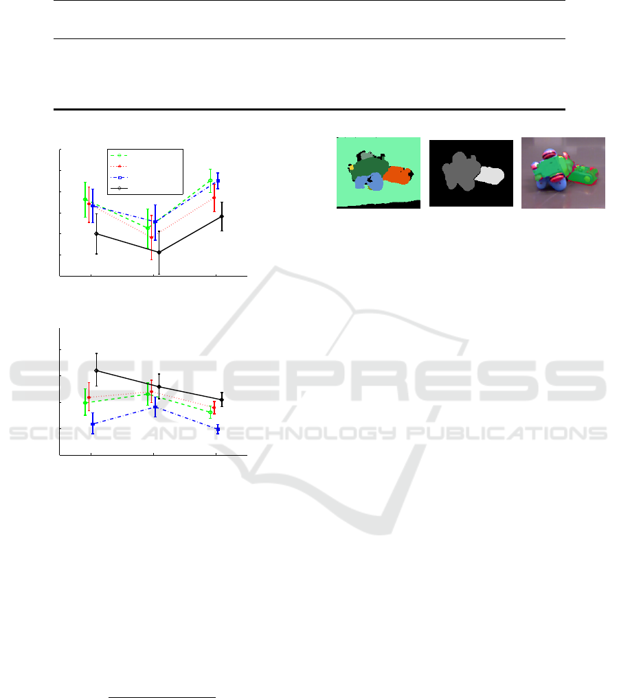
Table 2: True positive rate (tp) and false positive rate (fp) for each method. The best results, highest true positive rates and

lowest false positive rates, are bolded. In ”V4R one SVM” we have used only structural level SVM, and in ”V4R two SVMs”

we have used structural+assembly level SVMs, similarly as in (Richtsfeld et al., 2014).

tp fp

mean 95% conﬁdence interval mean 95% conﬁdence interval

V4R one SVM 0.6766 (0.6510, 0.7017) 0.1979 (0.1840, 0.2126)

V4R two SVMs 0.6556 (0.6286, 0.6816) 0.2065 (0.1924, 0.2220)

LCCP 0.6723 (0.6489, 0.6948) 0.1635 (0.1528, 0.1756)

ICL 0.5999 (0.5717, 0.6277) 0.2383 (0.2220, 0.2561)

2−4 toys 6−7 toys 14−18 toys

0.5

0.55

0.6

0.65

0.7

0.75

0.8

True positive rate

V4R−1SVM

V4R−2SVM

LCCP

ICL

(a) True positive rates

2−4 toys 6−7 toys 14−18 toys

0.1

0.15

0.2

0.25

0.3

False positive rate

(b) False positive rates

Figure 4: Results for different number of toys in test set

images, partitioned as in Table 1. The test set contained

126 images with 2-4 toys, 59 images with 6-7 toys and 63

images with 14-18 toys.

where S

assigned

is the set of pixels assigned to a given

object, and S

annotated

is the set of annotated pixels in

the ground truth image for that object. Hence, the true

positive rate for one object is the number of true posi-

tive pixels divided by the number of annotated pixels.

Likewise, the false positive rate f p for one object is

f p =

assigned

annotated

assigned

. (3)

The false positive rate is the ratio of assigned pixels

that do not coincide with the annotated pixels to the

number of assigned pixels in total.

Table 2 shows the results for each method when

the whole test set is used. From the results we see

that V4R’s segmenter and LCCP have the highest true

(a)

(b)

(c)

Figure 5: Example of a segmentation with two objects. (a)

shows the segmentation where each color corresponds to a

segmented object. The ground truth image (b) shows the

actual pixel labels. (c) shows the evaluation where transpar-

ent green highlights true positives and transparent red false

positives. In (a), several segmented objects overlap the ac-

tual object on the left. The evaluation procedure assigns the

segmented object with the most overlapping pixels to the

actual object: for the left object the object segmented with

dark green in (a).

positive rates on the test set, while LCCP has a lower

false positive rate than V4R. Figure 4 displays results

for each segmenter when we have divided the test set

into partitions according to how many toys there are in

the images. The conﬁdence intervals are the longest

in the set with 2-4 toys, because the impact of incor-

rectly segmenting objects is larger. For instance, if a

segmenter fails to segment both of two objects, the re-

sulting true positive rate for that image will be zero.

Then, if there are, say, 18 objects in an image and

the segmenter fails to segment 2 of those objects, the

true positive rate is still signiﬁcantly higher than zero.

This leads to higher variance in the results of images

with less toys, and hence longer conﬁdence intervals.

5 DISCUSSION

As expected, ICL did not fare well with the dataset’s

complex toys. What is surprising, however, is that

LCCP and V4R did equally well in the true positive

rate, and LCCP had signiﬁcantly lower false positive

rate than V4R. The low false positive rate is due to

comprehensive oversegmentation in the LCCP’s pre-

segmentation phase, which results in multiple non-

connected patches in some of the objects. This pre-

VISAPP 2016 - International Conference on Computer Vision Theory and Applications

114

vents the occurrence of false positives, as the seg-

mented pixels are always in the area of the annotated

ground truth pixels. However, it also lowers the true

positive rate since these patches are not connected to

the patch that is assigned to the object.

By examining the segmented images by each

method, we made a few observations. ICL failed

many of the objects completely by segmenting them

as part of the table, which reduces the true positive

rate signiﬁcantly. This happened to other methods as

well, though not so frequently. Furthermore, all the

methods often incorrectly joined two or three objects

together, which explains the high false positive rates.

Figure 3 demonstrates some of the aforementioned

observations for three different images from the toy-

dataset.

ICL’s poor results might originate from their

weighted similarity graph, which considers the ad-

jacency, curvature and coplanarity of found surface

patches. Out of these three attributes especially the

curvature and coplanarity incur problems, since many

of the presegmented surface patches are not symmet-

rical or similar. In other words, the shapes of the

patches differ from each other and they are not copla-

nar.

Table 2 contains results for V4R with one and two

SVMs, or structural and structural+assembly level

SVMs, as Richtsfeld et al. also used both methods on

OSD in their paper (Richtsfeld et al., 2014). It is not

obvious which method, one or two SVMs, performs

better in the OSD, for when using only one SVM the

precision is higher but recall is lower as opposed to

using two SVMs. In our dataset, however, using only

one SVM, the structural level SVM, seems to be a

preferred choice.

As we discussed in the beginning of Section 4,

a model-free method will perform poorly if its im-

plicit model of the objects is wrong. In this case it

seems that the implicit model of the convexity-based

LCCP is more appropriate to the toy-dataset than the

implicit model of ICL. It is also noteworthy that ICL

and V4R received similar results in the OSD, whereas

here V4R was more efﬁcient than ICL. It seems that

the implicit model of ICL is better suited to the kind

of objects found in OSD than the objects in the toy-

dataset.

In any event, there are some sources of errors that

affect the computed results. When viewing the point

clouds of the images, it is apparent that the RGB

and depth images are not completely aligned at some

places. Since the ground truth images are created

from the RGB images, the misalignment implies that

the segmented pixels cannot coincide with annotated

pixels of an object. This basically shifts some of true

positive pixels into false positive pixels, reducing the

true positive rate and increasing the false positive rate.

Also, there is often noise around the edges of the ob-

jects, which affects the true and false positive rates,

and further, there exists the already mentioned dif-

ﬁculties (Section 3.1) with annotation of the ground

truth images.

Regardless, the slight misalignment of color and

depth images, as well as the noisy observations of

the objects, reﬂect the commonplace problems of

a robot operating in the real world. Accordingly,

our dataset corresponds to real circumstances under

which a robot usually operates, along with the non-

ideal lighting conditions and a relatively poor quality

RGB-D sensor.

6 CONCLUSION

In this paper we presented a novel RGB-D dataset de-

signed for shifting the focus from relatively simple

objects to more complicated ones in the object seg-

mentation scene. The dataset contains 449 highly oc-

cluded images of 24 toys, which vary greatly in shape,

color and size, and contain minute texture.

Also, the toy-dataset provides a new benchmark

against which forthcoming segmenters can test their

performance. Our experiments demonstrated that the

V4R and LCCP segmenters performed equally well

on our dataset of toys, even though the model-based

V4R was trained using data from the toy-dataset. It

seems that the features used by V4R might need some

alteration to account for the complex objects in our

dataset. Furthermore, the actual goal of the LCCP

segmenter is to partition complex objects into parts,

which generates oversegmentation. This oversegmen-

tation however has both an upside and a downside, as

it lowers both false and true positive rates. Lastly, the

ICL segmenter seems to perform better on symmetri-

cal objects, such as boxes, bowls and cylinders found

in the OSD, but the asymmetric objects in our dataset

deteriotate the performance of the segmenter.

ACKNOWLEDGEMENTS

This work was supported by Academy of Finland, de-

cisions 264239 and 271394.

REFERENCES

Anand, A., Koppula, H. S., Joachims, T., and Saxena, A.

(2011). Contextually guided semantic labeling and

Benchmarking RGB-D Segmentation: Toy Dataset of Complex Crowded Scenes

115

search for 3D point clouds. International Journal of

Robotics Research, abs/1111.5358.

Burges, C. (1998). A tutorial on support vector machines

for pattern recognition. Data Mining and Knowledge

Discovery, 2(2):121–167.

Chang, C.-C. and Lin, C.-J. (2011). LIBSVM: A library

for support vector machines. ACM Transactions on

Intelligent Systems and Technology, 2(3):1–27.

Chen, Y.-W. and Lin, C.-J. (2006). Combining SVMs

with various feature selection strategies. In Feature

Extraction, volume 207 of Studies in Fuzziness and

Soft Computing, chapter 13, pages 315–324. Springer

Berlin Heidelberg.

Hinterstoisser, S., Lepetit, V., Ilic, S., Holzer, S., Brad-

ski, G. R., Konolige, K., and Navab, N. (2012).

Model based training, detection and pose estimation

of texture-less 3D objects in heavily cluttered scenes.

In Proceedings of the Asian Conference on Computer

Vision (ACCV), pages 548–562. Springer.

Koppula, H. S., Anand, A., Joachims, T., and Saxena, A.

(2011). Semantic labeling of 3D point clouds for in-

door scenes. In Advances in Neural Information Pro-

cessing Systems, pages 244–252. Curran Associates,

Inc.

Lai, K., Bo, L., Ren, X., and Fox, D. (2011). A large-scale

hierarchical multi-view RGB-D object dataset. In

Proceedings of the IEEE International Conference on

Robotics and Automation (ICRA), pages 1817–1824.

IEEE.

Mian, A., Bennamoun, M., and Owens, R. (2006). Three-

dimensional model-based object recognition and seg-

mentation in cluttered scenes. IEEE Transac-

tions on Pattern Analysis and Machine Intelligence,

28(10):1584–1601.

Mian, A., Bennamoun, M., and Owens, R. (2010). On the

repeatability and quality of keypoints for local feature-

based 3D object retrieval from cluttered scenes. In-

ternational Journal of Computer Vision, 89(2-3):348–

361.

Richtsfeld, A., M

orwald, T., Prankl, J., Zillich, M., and

Vincze, M. (2012). Segmentation of unknown ob-

jects in indoor environments. In Proceedings of

the IEEE/RSJ International Conference on Intelligent

Robots and Systems (IROS), pages 4791–4796. IEEE.

Richtsfeld, A., M

orwald, T., Prankl, J., Zillich, M., and

Vincze, M. (2014). Learning of perceptual group-

ing for object segmentation on RGB-D data. Journal

of Visual Communication and Image Representation,

25(1):64 – 73.

Rusu, R. B. and Cousins, S. (2011). 3D is here: Point

cloud library (PCL). In Proceedings of the IEEE In-

ternational Conference on Robotics and Automation

(ICRA), pages 1–4. IEEE.

Silberman, N. and Fergus, R. (2011). Indoor scene segmen-

tation using a structured light sensor. In Proceedings

of the IEEE International Conference on Computer

Vision (ICCV) Workshops, pages 601–608. IEEE.

Silberman, N., Hoiem, D., Kohli, P., and Fergus, R.

(2012). Indoor segmentation and support inference

from RGBD images. In Proceedings of the 12th Euro-

pean Conference on Computer Vision (ECCV), pages

746–760. Springer-Verlag.

Singh, A., Sha, J., Narayan, K. S., Achim, T., and Abbeel,

P. (2014). BigBIRD: A large-scale 3D database of

object instances. In Proceedings of the IEEE In-

ternational Conference on Robotics and Automation

(ICRA), pages 509–516. IEEE.

Stein, S., Schoeler, M., Papon, J., and Worgotter, F. (2014).

Object partitioning using local convexity. In Proceed-

ings of the IEEE Conference on Computer Vision and

Pattern Recognition (CVPR), pages 304–311. IEEE.

Uckermann, A., Haschke, R., and Ritter, H. (2013). Re-

altime 3D segmentation for human-robot interaction.

In Proceedings of the IEEE/RSJ International Confer-

ence on Intelligent Robots and Systems (IROS), pages

2136–2143. IEEE.

VISAPP 2016 - International Conference on Computer Vision Theory and Applications

116