Cornea-reﬂection-based Extrinsic Camera Calibration

without a Direct View

Kosuke Takahashi, Dan Mikami, Mariko Isogawa and Akira Kojima

NTT Media Intelligence Laboratories, Nippon Telegraph and Telephone Corporation,

1-1, Hikarinooka Yokosuka-Shi, Kanagawa, Japan

Keywords:

Camera Calibration, Cornea Reﬂection, Spherical Mirror.

Abstract:

In this paper, we propose a novel method to extrinsically calibrate a camera to a 3D reference object that is

not directly visible from the camera. We use the spherical human cornea as a mirror and calibrate the extrinsic

parameters from the reﬂections of the reference points. The main contribution of this paper is to present a

cornea-reﬂection-based calibration algorithm with minimal conﬁguration; there are ﬁve reference points on a

single plane and one mirror pose. In this paper, we derive a linear equation and obtain a closed-form solution

of extrinsic calibration by introducing two key ideas. The ﬁrst is to model the cornea as a virtual sphere,

which enables us to estimate the center of the cornea sphere from its projection. The second idea is to use

basis vectors to represent the position of the reference points, which enables us to deal with 3D information of

reference points compactly. Besides, in order to make our method robust to observation noise, we minimize

the reprojection error while maintaining the valid 3D geometry of the solution based on the derived linear

equation. We demonstrate the advantages of the proposed method with qualitative and quantitative evaluations

using synthesized and real data.

1 INTRODUCTION

Determining the geometric relationship between a

camera and a 3D reference object is called ex-

trinsic camera calibration, and has been a funda-

mental research ﬁeld in computer vision for many

years(Hartley and Zisserman, 2004; Zhang, 2000).

This technique is widely used as an essential element

of various applications, such as 3D shape reconstruc-

tion from multi-view images(Matsuyama et al., 2012;

Agarwal et al., 2010), and augmented reality(Azuma

et al., 2001). Conventional extrinsic calibration tech-

niques have a fundamental assumption: the camera

should observe the 3D reference object directly.

Display-camera systems such as laptop comput-

ers, smart phones, and digital signage have become

popular and thus gained much attention as a useful de-

vice for many tasks in computer vision. For example,

Hirayama et al.(Hirayama et al., 2010) estimate the

interest of users who are watching a digital signage.

They assume that the user’s gaze points represent

his/her interests in the displayed contents. As another

example, Kuster et al.(Kuster et al., 2012) propose a

gaze correction method with a display-camera setup

for home video conferences. For these applications,

they have to know the relative posture and position

Reference object (Display)

Calibrate



Captured cornea reﬂection image

Camera

Figure 1: Cornea-reﬂection-based extrinsic camera calibra-

tion. The goal of this paper is to calibrate the camera against

the reference object which lies out of the camera’s ﬁeld of

view.

of the camera against the display. However, the fun-

damental assumption of extrinsic camera calibration,

the camera should observe the 3D reference object di-

rectly, does not hold in some cases of display-camera

system calibration, as in (Hirayama et al., 2010) and

(Kuster et al., 2012). In this paper, we focus on ex-

trinsic camera calibration where the reference object

lies out of the camera’s ﬁeld of view.

If the reference object is hidden from the camera,

mirrors can be used to offset the occlusion. Some

studies on calibration with a mirror have described

setups to simplify calibration (Sturm and Bonfort,

2006; Kumar et al., 2008; Rodrigues et al., 2010;

Hesch et al., 2010; Nayar, 1997; Takahashi et al.,

2012; Agrawal, 2013; Francken et al., 2007; De-

Takahashi, K., Mikami, D., Isogawa, M. and Kojima, A.

Cornea-reﬂection-based Extrinsic Camera Calibration without a Direct View.

DOI: 10.5220/0005675300150024

In Proceedings of the 11th Joint Conference on Computer Vision, Imaging and Computer Graphics Theory and Applications (VISIGRAPP 2016) - Volume 3: VISAPP, pages 17-26

ISBN: 978-989-758-175-5

launoy et al., 2014). Techniques include decreas-

ing the number of required reference points or mir-

ror poses, because a simpler setup offers many advan-

tages for more robust calibration and lower computa-

tional cost. Takahashi et al.(Takahashi et al., 2012)

and Hesch et al.(Hesch et al., 2010) proposed calibra-

tion algorithms with three reference points and three

poses of a planar mirror, which is the minimal setup

for planar mirrors. To decrease the number of mir-

ror poses, Agrawal(Agrawal, 2013) proposed an al-

gorithm with one pose of a spherical mirror and eight

reference points. As a calibration method with no

additional hardware, Nitschke et al.(Nitschke et al.,

2011) used the cornea as a spherical mirror. This

method needs three reference points and both cornea

spheres, i.e., two spherical mirror poses.

In this paper, we focus on cornea-reﬂection-based

extrinsic camera calibration for occluded reference

objects (Figure 1). The contribution of this paper is to

present a calibration algorithm with minimal conﬁgu-

ration, that is ﬁve reference points on a single plane

and one spherical mirror (cornea sphere) pose. In this

paper, we derive a linear equation for estimating ex-

trinsic parameters by introducing two key ideas. The

ﬁrst is to model the cornea as a virtual sphere, which

enables us to estimate the center of the cornea sphere

from its projection. The second is to represent the po-

sition of reference points with basis vector expression,

which enables us to treat 3D information of the refer-

ence points compactly. By solving this linear equa-

tion, we obtain extrinsic parameters under the mini-

mal conﬁguration in a linear manner. Besides, in or-

der to make our method robust to observation noise,

we minimize the reprojection error while maintaining

the valid 3D geometry of the solution based on the

derived linear equation.

The rest of this paper is organized as follows. Sec-

tion 2 provides a review of conventional techniques

that use mirrors for calibration and clariﬁes the nov-

elty of the proposed method. Section 3 describes a

measurement model for calibration ﬁrst, and then in-

troduces key constraints and the algorithm. Section

4 details evaluations conducted on synthesized data

and real data to demonstrate the performance of our

method. Section 5 provides the discussions on the ef-

fects of noise on the cornea model and the validity of

using reprojection error as a criteria for detecting a

local minimum. Section 6 concludes this paper.

2 RELATED WORK

This section reviews conventional mirror-based cal-

ibration approaches and clariﬁes the contribution of

this paper. Mirror-based calibration algorithms that

use indirect observations of 3D reference objects can

be categorized in terms of the mirror shape, the num-

ber of minimal reference points and mirror poses (See

Table 1). First, we categorize them into two groups in

terms of mirror shape: (1) Planar mirrors (Sturm and

Bonfort, 2006; Kumar et al., 2008; Rodrigues et al.,

2010; Hesch et al., 2010; Nayar, 1997; Takahashi

et al., 2012), and (2) Spherical mirrors (Agrawal,

2013).

Planar Mirrors: The conventional methods in

this group can be categorized based on whether the

mirror duplicates the camera (mirrored camera ap-

proach) or the reference points (mirrored point ap-

proach). Hesch et al.(Hesch et al., 2010) take the

mirrored camera approach. They estimate the extrin-

sic parameters between the mirrored camera and the

true reference points (not reﬂections) by solving the

P3P problem(Haralick et al., 1994). They use them

for estimating the extrinsic parameters between the

camera and the true reference points with the con-

ﬁguration of three reference points and three mirror

poses. On the other hand, Takahashi et al.(Takahashi

et al., 2012) adopt the mirrored point approach. They

introduce an orthogonality constraint that should be

satisﬁed by all families of reﬂections of a single ref-

erence point and utilize it to estimate extrinsic param-

eters with the same conﬁguration. Note that Sturm

and Bonfort(Sturm and Bonfort, 2006) revealed that

at least three mirror poses are required to uniquely

determine the extrinsic parameters if the mirror is pla-

nar. Therefore, three reference points and three mirror

poses is the minimal conﬁguration for planar mirror

based methods.

Spherical Mirrors: Agrawal(Agrawal, 2013)

proposed a spherical mirror based calibration method.

They obtain an E matrix similar to the essential ma-

trix, by using a coplanarity constraint with eight point

correspondences and retrieve the extrinsic parameters

from the matrix.

Nitschke et al.(Nitschke et al., 2011) proposed a

method for calibrating display-camera setups from

the reﬂections in the user’s eyes (corneas) with no

additional hardware. They estimate 3D positions of

the reference points by ﬁnding the intersection of two

rays connecting a reference point to the center of the

eye ball. Their method needs three reference points

and both eyes, i.e., two spherical mirrors.

Our novel calibration method is also based on

cornea reﬂections because eliminating additional

hardware for calibration is important for casual

display-camera systems, such as webcams and smart-

phones. In this paper, we propose a calibration algo-

rithm that assumes the minimal conﬁguration of ﬁve

VISAPP 2016 - International Conference on Computer Vision Theory and Applications

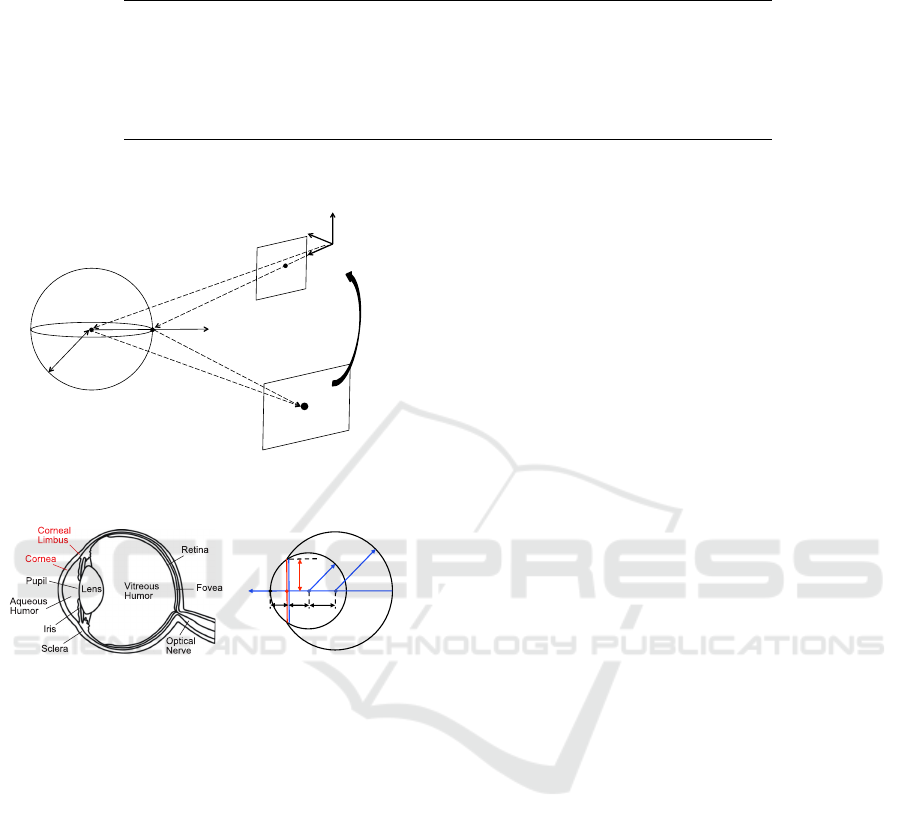
Table 1: Conﬁguration for each method: shape of mirrornumber of reference points and number of mirror poses.

Shape Points Poses

Kumar et al.(Kumar et al., 2008) Plane 5 3

Rodorigues et al.(Rodrigues et al., 2010) Plane 4 3

Hesch et al.(Hesch et al., 2010) Plane 3 3

Takahashi et al.(Takahashi et al., 2012) Plane 3 3

Agrawal (Agrawal, 2013) Sphere 8 1

Nitschke et al.(Nitschke et al., 2011) (Cornea) Sphere 3 2

Proposed (Cornea) Sphere 5 1

x

y

z

i

S

O

i

Sphere S (Corneal Sphere)

Reference Object X (Display)

Image Plane I

r

i

R,T

Camera C

Figure 2: Reﬂection model of spherical mirror.

      

S

E

A

E



Optical

Axis

Eyeball

Sphere

Corneal

Sphere

Cornea

AL

LS

SE

L

Corneal

Limbus

L

Iris

Figure 3: (a) Cross section(b) Geometric eye model based

on (Nakazawa and Nitschke, 2012).

reference points on a single plane and one pose of

a spherical mirror (cornea sphere) by introducing a

cornea sphere model and basis vector expression.

3 EXTRINSIC CAMERA

CALIBRATION USING

CORNEA REFLECTION

This section introduces our cornea reﬂection based

calibration algorithm; it determines the extrinsic pa-

rameters representing the geometric relationship be-

tween the camera and an obscured planar reference

object.

As illustrated by Figure 2, we assume that ref-

erence object X (Display) is located out of camera

C’s ﬁeld-of-view and there are N

reference points

(i = 1,··· , N

) on X. These reference points p

are mirrored by the eye ball and projected onto image

plane I as q

. Extrinsic parameters (rotation matrix R

and translation vector T ), which transform the refer-

ence object coordinate system {X} into the camera

coordinate system {C}, satisfy the following equa-

tion.

= Rp

{X}

+ T , (1)

where p

{X}

denotes the 3D position of p in {X }. We

assume that {C}is the world coordinate system in this

paper and omit this superscript if vector p is repre-

sented in {C}. Our goal is to estimate extrinsic pa-

rameters R and T from the projections of the reference

points.

3.1 Measurement Model based on

Cornea Reﬂection

In this section, we deﬁne the measurement model

based on the geometric relationship that holds when

treating the human eye ball as a spherical mirror.

The human eyeball can be modeled as two over-

lapping spheres as illustrated by Figure 3. Since

the reﬂections of reference points can be seen at the

cornea, we utilize the cornea sphere as a spherical

mirror whose center is S and radius is r.

As illustrated by Figure 2, m

denotes the reﬂec-

tion point of reference point p

on the cornea sphere.

Suppose the unit vector from the camera center O to

and unit vector from m

to p

are expressed as v

and u

, respectively, p

is expressed as follows:

= k

+ m

, (2)

where k

denotes the distance between m

and p

Based on the laws of reﬂection, u

is expressed as,

= v

+ 2(−v

·n

, (3)

where n

denotes the normal vector at m

. Since the

normal vector n

is the unit vector from the center of

cornea sphere S to m

, n

is expressed as n

= (m

−

S)/|m

−S|.

With the unit vector v

, m

is expressed as,

= k

, (4)

where k

denotes the distance between O and m

. By

using projection q

, we obtain v

= (K

−1

)/|K

−1

Cornea-reﬂection-based Extrinsic Camera Calibration without a Direct View

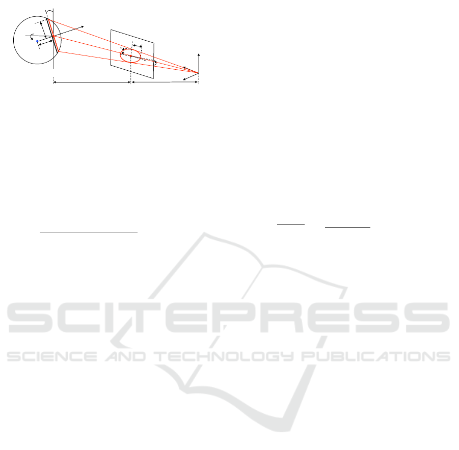
y

z

O

Camera C

Corneal!

Sphere

Average Depth Plane

d

f

max

min

L

φ

Projected Limbus

Image Plane

Gaze Direction g

Limbus

Iris

S

LS

φ

τ

L

x

Figure 4: Estimating the center of the cornea sphere from

limbus projection.

where matrix K denotes the intrinsic parameters and

supposed to be given beforehand.

Since m

is on the cornea sphere, m

satisﬁes |m

−

S| = r. By substituting Eq (4) for this equation and

multiplying it by itself, we have

−2k

S + |S|

−r

= 0, (5)

Solving Eq (5) yields two solutions such as k

S ±

−|v

(|S|

−r

))/|v

. Since m

the point closer to the camera among the intersections

of v

and the sphere surface, the smaller k

represents

the distance between O and m

By substituting Eq (2) into Eq (1), we obtain the

following equation:

{X}

+ T = k

+ m

. (6)

In this paper, we deﬁne Eq (6) as the measurement

model.

3.2 Reducing Unknown Parameters in

Measurement Model

Since only p

{X}

is known in Eq (6), we can not solve

Eq (6) and obtain extrinsic parameters by simply in-

creasing the number of reference points. In order to

reduce the unknown parameters, we introduce two

ideas (1) a geometric model of the cornea sphere and

(2) basis vector expression to represent 3D reference

point position, and propose an extrinsic calibration

method with minimal conﬁguration, that is ﬁve ref-

erence points and one mirror pose.

3.2.1 The Geometric Model of Cornea Sphere

In this section, we describe a method to estimate

the center of the cornea sphere, S, from limbus pro-

jection by introducing a geometric model(Nakazawa

and Nitschke, 2012). The average radius of the

cornea sphere, r, and the average radius of the

cornea limbus, r

, are 7.7 mm and 5.6 mm respec-

tively(Richard S.Snell, 1997).

As illustrated in Figure 4, the limbus projection

is modeled as an ellipse represented by ﬁve param-

eters: the center, i

, the major and minor radii, r

max

and r

min

, respectively, and rotation angle φ. Since the

depth variation of a tilted limbus is much smaller than

the distance between camera and the cornea sphere,

we assume the weak perspective projection. Un-

der this assumption, the 3D position of the center

of limbus L is expressed as L = dK

−1

, where d

denotes the distance between the center of the cam-

era O, and the center of the limbus L, and is ex-

pressed as d = f ·r

max

. f and K represent the fo-

cal length in pixels and intrinsic parameters, respec-

tively. Gaze direction g is approximated by the op-

tical axis of the eye, and is theoretically determined

by g = [sinτsin φ,−sin τcos φ,−cosτ]

, where τ =

±arccos(r

min

max

); τ corresponds to the tilt of the

limbus plane with respect to the image plane. Since

the center of cornea sphere, S, is located at distance

−r

√

7.7

−5.6

≈ 5.3mm) form the

limbus, the radius of the cornea sphere from L, we

compute S as follows,

S = L −d

g. (7)

In this way, we estimate S from the ellipse param-

eters of the limbus projected onto the image plane,

that is (i

,φ, r

max

min

From the above, by introducing the geometric

model of the cornea sphere, we can obtain unknown

parameters r and S in Eq (6).

3.2.2 Using Basis Vector Representation of 3D

Reference Point Position

In this paper, basis vector representation means rep-

resenting vector p as the linear combination of ba-

sis vectors, that is p = Σ

−1

j=0

, where e

( j =

0··· , N

−1) denotes the basis vector of N

dimen-

sional vector space and is independent linearly, and

is the coordinate of p with respect to the basis e

Here, we assume a three dimensional vector space,

that is N

= 3. With this basis vector representation,

in the reference object coordinate system {X } is

expressed as,

{X}

= Σ

j=0

i{X}

{X}

, (8)

where a

i{X}

denotes the coordinates of p

{X}

with re-

spect to basis e

{X}

. By assuming p

{X}

and e

{X}

are

given a priori, a

i{X}

can be computed. By substituting

Eq (8) into Eq (1), we have

= Σ

j=0

i{X}

{X}

+ T . (9)

VISAPP 2016 - International Conference on Computer Vision Theory and Applications

In cases where p

{X}

represents the origin of the refer-

ence object coordinate system, p

can be considered

as translation vector T. Therefore p

can be expressed

as follows

= Σ

j=0

i{X}

{X}

+ p

. (10)

3.3 Derivation of Linear Equation for

Estimating Extrinsic Parameters

In this section, we derive a linear equation for esti-

mating extrinsic parameters by using two ideas intro-

duced in Section 3.2.1 and 3.2.2.

By substituting Eq (10) into Eq (6) and represent-

ing p

by using Eq (2), we have

j=0

i{X}

{X}

+ k

+ m

= k

+ m

(11)

We deﬁne each basis vector as e

{X}

[1,0, 0]

{X}

= [0,1,0]

{X}

= [0,0,1]

. From Eq

(11) for the N

reference points, we can derive the

following linear equation:

AX = B, (12)

where,

A =







−1







(13)

= a

i{X}

3×3

, (14)

··· w

−1

, (15)



−u

(l = m)

3×1

(otherwise)



, (16)

X =



··· k

−1



(17)

B =



··· m

−1



, (18)

= (m

−m

)

. (19)

Vectors r

, r

and r

denote the ﬁrst, second and third

columns of the rotation matrix R = [r

In this paper, we assume that we use a planar

display as the reference object, that is the reference

points lie on the same planea. In this case, a reference

point in the reference object coordinate system can be

expressed as p

{X}

= (x

,0) and all a

are zero. By

removing r

, which is the unknown parameter cor-

responding to a

in Eq (12), we have the following

linear equation:

= B, (20)

where







−1







, (21)



··· k

−1



. (22)

With N

reference points, we have (6 + N

) un-

knowns (X

) and 3(N

−1) constraints (rows of A

and

B) in Eq (20). Hence, when N

≥ 5, we can solve Eq

(20) by X

= A

0∗

B, where A

0∗

is the pseudo-inverse

matrix of A

. r

is given by the cross product of r

and r

, i.e. r

= r

×r

In real environment, the rotation matrix R =

] obtained by solving Eq (20) is not guaranteed

to satisfy the constraints to form a valid rotation ma-

trix (| r

|=| r

|= 1,r

= r

= 0).

In order to enforce these constraints, here we solve the

orthogonal Procrustes problem (Golub and van Loan.,

1996) as done by Zhang’s method (Zhang, 2000).

This linear solution estimates the correct extrin-

sic parameters in noiseless environments. As shown

in Figure 6, we can see that extrinsic parameter pre-

cision degrades remarkably if the input data includes

observation noise (We describe the experimental en-

vironment in detail in Section 4). To overcome this

difﬁculty, we solve the non-linear optimization prob-

lem of the objective function derived from Eq (20),

which is robust to noise.

3.4 Solving Non-linear Optimization

Problem

3.4.1 Objective Function

We deﬁne an objective function for non-linear opti-

mization with two error terms. First, we introduce an

error term for the measurement model. Ideal extrin-

sic parameters should satisfy the linear equation of Eq

(20), which is derived from the measurement model.

In order to enforce this constraint on the estimated ex-

trinsic parameters, we introduce the following error

term,

cost

model

(R,T ) = |A

(R,T ) −B|, (23)

where X

(R,T ) denotes X

computed from the esti-

mated R and T .

Second, we introduce an error term to minimize

the reprojection error as widely done in the calibration

(Triggs et al., 2000):

Cornea-reﬂection-based Extrinsic Camera Calibration without a Direct View

!"#$%&'()*+#%,(-%,.'

!"#$%&'('/&0+*"+1(2%0%$'&'0"(34("5,6+*7(

*5*8,+*'%0(,'%"&("9.%0'"(2053,'$"(5:(!9(;<=>(

?2@%&'()*+#%,(-%,.'

No

Yes

A&%0&

!*@

cost

rep

(R,T) / N

< t

rep

Figure 5: Implementation strategy.

cost

rep

(R,T ) =

−1

∑

i=0

− ˘q

(R,T )|, (24)

where ˘q

(R,T ) denotes q

calculated from the esti-

mated R and T .

By introducing these error terms, we deﬁne the

following objective function f ,

f = c

model

∗cost

model

(R,T )

+ c

rep

∗cost

rep

(R,T ),

(25)

where c

model

and c

rep

are the coefﬁcients correspond-

ing to cost

model

and cost

rep

respectively.

3.4.2 Implementation

We implement our proposed method together with

non-linear optimization as illustrated in Figure 5.

First, we estimate the initial values of extrinsic param-

eters. In this paper, we use a linear solution of extrin-

sic parameters estimated by solving Eq (20) as the ini-

tial value. Second, we use the Levenberg-Marquardt

algorithm to solve the non-linear optimization prob-

lem of Eq (25). However, Eq (25) is not a convex

function and it can converge to a local minimum.

Against this problem, we use the reprojection error as

the criteria indicating whether the estimated solution

is a local minimum or not. When the average repro-

jection error cost

rep

(R,T )/N

is larger than a thresh-

old t

rep

, that is the estimated solution is a local mini-

mum, we update the initial value of extrinsic param-

eters by adding random values and resolve the non-

linear optimization problem until cost

rep

(R,T )/N

rep

is satisﬁed.

4 EXPERIMENT

This section details the experiments conducted on

synthesized and real data in order to evaluate

the quantitative and qualitative performance of our

method. In the following, “linear solution” denotes

extrinsic parameters estimated by solving Eq (20)

in linear manner and “non-linear solution” denotes

those estimated by solving the non-linear optimiza-

tion problem of Eq (25).

4.1 Synthesized Data

4.1.1 Experiment Environment

The synthesized data was generated as follows. The

matrix of the intrinsic parameters, K, consists of

( f x, f y,cx,cy); f x and f y represent the focal length

in pixels, and cx and cy represent the 2D coor-

dinates of the principal point. We set them to

(1400,1400, 960,540) in this evaluation respectively.

We set the camera coordinate system as the

world coordinate system and set the center of cam-

era to O = (0,0,0). The 3D positions of the ref-

erence points are deﬁned as p

{X}

= (0, 0,0), p

{X}

(−50,50, 0), p

{X}

= (50,50, 0), p

{X}

= (−50,−50,0)

and p

{X}

= (50,−50,0). The center of the cornea

sphere is set to S = (0,45,50), the d

is set to

5.6mm and radius r is set to 7.7mm on the basis of

(Richard S.Snell, 1997).

We represent the ground truth of R as the product

of three elemental matrices, one for each axis, that

is R = R

(θ

), and we set (θ

,θ

) to

(−0.1,0.2, 0)[rad]. The ground truth of T is set to

(0,90, 0). In the optimization process, c

model

rep

and

dist

are set to 1 and t

rep

is set to 2.

Throughout this experiment, we evaluate the dis-

tance between estimated parameter and its ground

truth, and reprojection error as error metrics. Here,

parameters with subscript g indicate ground truth

data. The distance between R and R

, D

(R,R

), is

deﬁned as the Riemannian distance (Moakher, 2002):

√

k Log(R

) k

, (26)

LogR

(

0 (θ = 0),

2sinθ

−R

) (θ 6= 0),

(27)

where θ = cos

−1

(

trR

−1

). The difference between T

and T

, D

(T ,T

), is deﬁned as RMS:

| T −T

/3. (28)

The reprojection error is deﬁned as D

cost

rep

(R,T )/N

In this simulation, we computed linear and non-

linear solutions from the projection of reference

point q

with zero-mean Gaussian noise whose stan-

dard deviation σ

(0 ≤ σ

≤ 1). We compared our

method against the state-of-the-art of planar mir-

ror based method proposed by Takahashi(Takahashi

et al., 2012). For fair comparison, the projections of

reference points using either spherical or planar mir-

rors are assured to occupy a comparable pixel area in

the image as done in (Agrawal, 2013).

VISAPP 2016 - International Conference on Computer Vision Theory and Applications

0 0.2 0.4 0.6 0.8 1

Student Version of MATLAB

0 0.2 0.4 0.6 0.8 1

Student Version of MATLAB

0 0.2 0.4 0.6 0.8 1

0.5

1.5

Student Version of MATLAB

p

R

T

Reprojection Error

noise σ

(pixel)

noise σ

(pixel)

Error of Rotation Matrix Error of Translation Vector

noise σ

(pixel)

Proposed (linear)

Takahashi et al

Proposed (linear)

Takahashi et al

Proposed (linear)

Takahashi et al

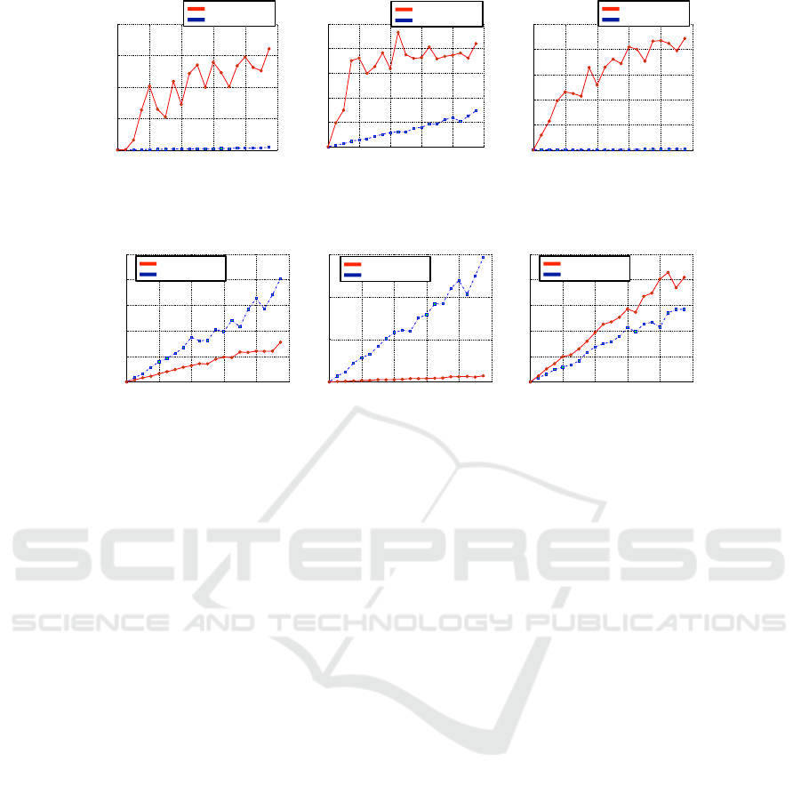
Figure 6: Estimation errors of linear solution under Gaussian noise for q

with standard deviation σ

0 0.2 0.4 0.6 0.8 1

0.01

0.02

0.03

0.04

0.05

Student Version of MATLAB

0 0.2 0.4 0.6 0.8 1

Student Version of MATLAB

0 0.2 0.4 0.6 0.8 1

0.1

0.2

0.3

0.4

0.5

Student Version of MATLAB

Proposed (non-linear)

Takahashi et al

Reprojection Error

noise σ

(pixel)

noise σ

(pixel)

Error of Rotation Matrix Error of Translation Vector

noise σ

(pixel)

Proposed (non-linear)

Takahashi et al

Proposed (non-linear)

Takahashi et al

p

R

T

Figure 7: Estimation errors of non-linear solution under Gaussian noise for q

with standard deviation σ

4.1.2 Results with Synthesized Data

Figure 6 and Figure 7 show D

and D

of the lin-

ear solution and the non-linear solution respectively.

In each ﬁgure, the vertical axis shows the average

value over 50 trials and the horizontal axis denotes

the standard deviation of noise.

Linear Solution. From Figure 6, we can observe

that D

and D

are zero at σ = 0, which means

that the minimal conﬁguration of our method, that is

ﬁve reference points and one mirror pose, is sufﬁcient.

However, when σ

> 0, D

and D

increase re-

markably. Additionally, most estimated T values, that

is p

, are located around the surface of the cornea

sphere. This is explained as follows: In the proposed

algorithm, we estimate the linear solutions of R and

T as the parameters X

that minimizes ||A

−B||

Since the cornea has a very small radius, unit vector u

used in A

changes signiﬁcantly with even trivial ob-

servation noise. If u

is wrong, ||A

−B||

increases

with the distance between reference points and their

reﬂection points on the surface of the spherical mir-

ror, that is k

in X

. Therefore, in cases where the

input data includes observation noise, it is considered

that ||A

−B||

is minimized with small k

, which

means T is located around the surface of the cornea

sphere.

Non-linear Solution. From Figure 7, we

can observe that estimation errors D

and

are signiﬁcantly smaller than those of

Takahashi et al.(Takahashi et al., 2012)

(57.5%,94.7%,respectively). These results quantita-

tively prove that our method outperforms Takahashi

et al.(Takahashi et al., 2012) and works robustly even

if the input data includes observation noise.

4.2 Real Data

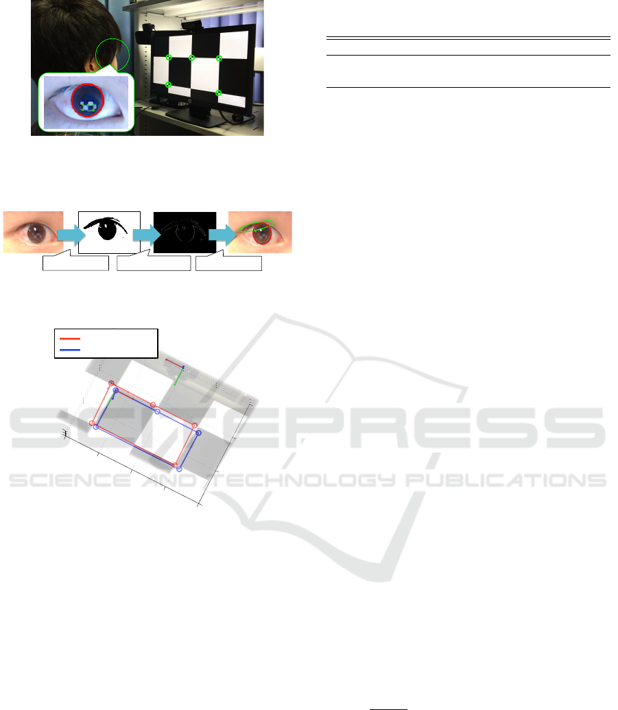
4.2.1 Conﬁguration

Figure 8 overviews the conﬁguration. We used a

Logicool HD Pro Webcam C920t and captured frames

had the resolution of 1920 ×1080. As illustrated

in Figure 8, we projected a chessboard pattern on

the display and captured the cornea as the reference

points p

(i = 0,··· , 4). The size of each chess block

was 125 ×125mm. The distance between the user’s

cornea center and the display was about 300 mm.

The intrinsic parameter was estimated beforehand by

(Zhang, 2000). In order to estimate ellipse parameters

,φ, r

max

min

) from limbus projection, we binarize

the input image, apply the Canny detector and ﬁt an

ellipse (Fitzgibbon and Fisher, 1995) as shown in Fig-

ure 9.

Since the ground truth of extrinsic parameters is

not available in any real conﬁguration, we used (Taka-

hashi et al., 2012) as the reference parameters.

Cornea-reﬂection-based Extrinsic Camera Calibration without a Direct View

Camera 

3

0

2

Reference Point



0

1

4



2

3

4

Figure 8: Conﬁguration for experiments with real data. No-

tice that we use only ﬁve points p

(i = 0, ··· , 4) of the chess-

board pattern as the reference points for calibration. Each

is separated by about 10 ∼ 13 pixels in captured image.

Binalization

Canny detector

Fit ellipse

Figure 9: A ﬂow of estimating ellipse parameters

,φ,r

max

min

) from projection of limbus.

−200

−100

100

200

100

200

300

−100

100

Student Version of MATLAB

Proposed (non-linear)

Takahashi et al

Camera

Reference Point

0

1

2

3

4

Figure 10: Positions of the reference points as estimated by

proposed method (red), by (Takahashi et al., 2012) (blue).

4.2.2 Results with Real Data

Table 2 quantitatively compares the parameters esti-

mated by the proposed method (linear solution and

non-linear solution) with (Takahashi et al., 2012).

We can see that the distance functions yielded

by the linear solution output large differences. It is

considered that some observation noise is present be-

cause the estimated T is close to surface of the cornea

sphere.

On the other hand, the non-linear solution yields

small differences. This point can be veriﬁed by vi-

sualizing the results as shown in Figure 10. It shows

that the positions estimated by the proposed method

are almost identical to those of (Takahashi et al.,

2012). This conﬁrms that our method works prop-

erly in real environments. While this precision may

not by enough for eye gaze tracking, it is acceptable

Table 2: Error metrics computed by using (Takahashi et al.,

2012) as the ground truth.

Linear solution 0.553 178.896 14.689

Non linear solution 0.164 33.617 0.260

for applications that do not need high precision, such

as gaze correction (Kuster et al., 2012) using a display

and attached web camera system.

5 DISCUSSION

In this section, we discuss the effects of noise on the

cornea model used in the proposed method and the

validity of using the reprojection error as the criteria

for detecting local minimum.

5.1 Effects of Differences Among

Individuals

In our porposed method, we have two assumptions

about the cornea model. The ﬁrst assumption is the

radius of cornea sphere r. While we use the aver-

age radius of the cornea sphere, that is r = 7.7mm

(Richard S.Snell, 1997), it can vary with the individ-

ual. The second one is the radius of cornea limbus

. In this paper we use the average size r

= 5.6mm,

but in practice the model parameters can be tailored

to suit the individual. To more closely examine the

effects of these assumptions, we investigated the ef-

fects of noise on these two radii with synthesized

data. We used the same conﬁguration as in Section

4.1 and set t

rep

to 10. We added random noise with

uniform distribution n

and n

to r and r

, respec-

tively, (0 ≤ |n

| ≤ 1,0 ≤|n

| ≤ 1).

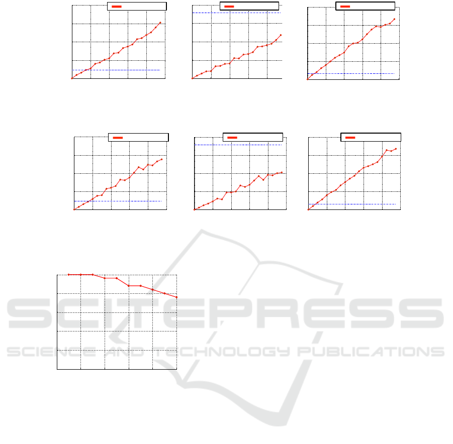
Figure 11 and Figure 12 show the results of the

averages of each distance function and reprojection

error. From Figure 11 and Figure 12, we can see that

r and r

have strong and similar impact to the esti-

amtion error of extrinsic parameters and reprojection

error. This because adding noise to r and r

affects

the precisions of S estimation based on Eq (7) and

−r

, and the direction and location of the

reﬂection on the cornea sphere changes signiﬁcantly

depending on S and r. To solve this problem, it is use-

ful to calibrate the user’s eye parameters beforehand.

VISAPP 2016 - International Conference on Computer Vision Theory and Applications

0 0.2 0.4 0.6 0.8 1

0.1

0.2

0.3

0.4

Student Version of MATLAB

0 0.2 0.4 0.6 0.8 1

Student Version of MATLAB

0 0.2 0.4 0.6 0.8 1

Student Version of MATLAB

Reprojection Error

noise n

(mm)

p

noise n

(mm)

R

Error of Rotation Matrix Error of Translation Vector

T

noise n

(mm)

Proposed (non-linear)

(reference data: Takahashi et al (σ

= 1))

(reference data: Takahashi et al (σ

= 1))

(reference data: Takahashi et al (σ

= 1))

Proposed (non-linear)

Figure 11: Estimation errors under random noise for radius of cornea sphere r with uniform distribution.

0 0.2 0.4 0.6 0.8 1

0.1

0.2

0.3

0.4

Student Version of MATLAB

0 0.2 0.4 0.6 0.8 1

Student Version of MATLAB

0 0.2 0.4 0.6 0.8 1

Student Version of MATLAB

Reprojection Error

noise n

(mm)

p

noise n

(mm)

R

Error of Rotation Matrix Error of Translation Vector

T

noise n

(mm)

Proposed (non-linear)

(reference data: Takahashi et al (σ

= 1))

(reference data: Takahashi et al (σ

= 1))

(reference data: Takahashi et al (σ

= 1))

Proposed (non-linear)

Figure 12: Estimation errors under random noise for radius of cornea limbus r

with uniform distribution.

0 2 4 6 8 10

100

Student Version of MATLAB

rep

(pixel)



The rate of obtaining!

ground truth (%)

Figure 13: The rate of matching ground truth for each t

rep

5.2 Validity of using Reprojection Error

as the Criteria for Detecting Local

Minimum

In Section 3.4.2, we use the reprojection error as the

metric indicating whether the estimated solution is a

local minimum or not. Here we address the validity

of this usage by referring to simulation data. In the

simulation, we investigate the rate with which we can

match the ground truth in cases where the reprojection

error is smaller than t

rep

(1 ≤t

rep

≤ 10). Note that we

regarded the estimated R and T as matching to the

ground truth if D

< t

and D

< t

, which are

set to t

= 0.02 and t

= 6 respectively based on

the result of (Takahashi et al., 2012) with σ

= 0.5.

We use the same conﬁguration as in Section 4.1. We

added Gaussian noise with zero mean and standard

deviation σ

= 0.5 to q

Figure 13 shows the rate of matching the ground

truth for each t

rep

over 50 trials. From Figure 13, we

can observe that all the estimated solutions conver-

gence to the ground truth when t

rep

≤ 3. These simu-

lation results conﬁrm that using the reprojection error

as the metric for detecting the local minimum is valid

in practice. Based on this result, we deﬁne t

rep

= 2 in

Section 4. However, the relationship between σ

and

rep

is not proven theoretically. This is a part of future

work of this study.

6 CONCLUSION

In this paper, we proposed a new algorithm that cal-

ibrates a camera to a 3D reference object via cornea

reﬂection with the minimal conﬁguration. The key

ideas of our method are to introduce a geometric

cornea model and to use basis vector expression to

represent the 3D positions of reference points. Based

on these ideas, we derived a linear equation and ob-

tained a closed-form solution. Additionally, based on

the linear equation, we obtained a non-linear solution

that is robust to observation noise. In evaluations, our

method outperformed a state-of-the-art of planar mir-

ror based method with both synthesized and real data.

Cornea-reﬂection-based Extrinsic Camera Calibration without a Direct View

REFERENCES

Agarwal, S., Furukawa, Y., Snavely, N., Curless, B., Seitz,

S. M., and Szeliski, R. (2010). Reconstructing rome.

IEEE Computer, 43:40–47.

Agrawal, A. (2013). Extrinsic camera calibration without a

direct view using spherical mirror. In Proc. of ICCV.

Azuma, R., Baillot, Y., Behringer, R., Feiner, S., Julier, S.,

and MacIntyre, B. (2001). Recent advances in aug-

mented reality. Computer Graphics and Applications,

IEEE, 21(6):34 –47.

Delaunoy, A., Li, J., Jacquet, B., and Pollefeys, M. (2014).

Two cameras and a screen: How to calibrate mobile

devices? In 3D Vision (3DV), 2014 2nd International

Conference on, volume 1, pages 123–130. IEEE.

Fitzgibbon, A. and Fisher, R. B. (1995). A buyer’s guide to

conic ﬁtting.

Francken, Y., Hermans, C., and Bekaert, P. (2007). Screen-

camera calibration using a spherical mirror. In 4th

Canadian Conference on Computer and Robot Vision.

Golub, G. and van Loan., C. (1996). Matrix Computa-

tions. The Johns Hopkins University Press, Baltimore,

Maryland, third edition.

Haralick, B. M., Lee, C.-N., Ottenberg, K., and N

olle, M.

(1994). Review and analysis of solutions of the three

point perspective pose estimation problem. IJCV,

13:331–356.

Hartley, R. I. and Zisserman, A. (2004). Multiple View Ge-

ometry in Computer Vision. Cambridge University

Press, second edition.

Hesch, J., Mourikis, A., and Roumeliotis, S. (2010). Mirror-

based extrinsic camera calibration. In Algorithmic

Foundation of Robotics VIII, volume 57, pages 285–

299.

Hirayama, T., Dodane, J.-B., Kawashima, H., and Mat-

suyama, T. (2010). Estimates of user interest using

timing structures between proactive content-display

updates and eye movements. IEICE Trans. Informa-

tion and Systems, 93(6):1470–1478.

Kumar, R., Ilie, A., Frahm, J.-M., and Pollefeys, M. (2008).

Simple calibration of non-overlapping cameras with a

mirror. In Proc. of CVPR.

Kuster, C., Popa, T., Bazin, J.-C., Gotsman, C., and Gross,

M. (2012). Gaze correction for home video confer-

encing. ACM Trans. Graph., 31(6):174:1–174:6.

Matsuyama, T., Nobuhara, S., Takai, T., and Tung, T.

(2012). 3D Video and Its Applications. Springer Pub-

lishing Company, Incorporated.

Moakher, M. (2002). Means and averaging in the group of

rotations. SIAM J. Matrix Anal. Appl., 24:1–16.

Nakazawa, A. and Nitschke, C. (2012). Point of gaze esti-

mation through corneal surface reﬂection in an active

illumination environment. In Proc. of ECCV.

Nayar, S. (1997). Catadioptric omnidirectional camera. In

Proc. of CVPR.

Nitschke, C., Nakazawa, A., and Takemura, H. (2011).

Display-camera calibration using eye reﬂections and

geometry constraints. CVIU, 115(6):835 – 853.

Richard S.Snell, M. A. L. (1997). Clinical Anatomy of the

Eye. Wiley-Blackwell, second edition.

Rodrigues, R., Barreto, P., and Nunes, U. (2010). Camera

pose estimation using images of planar mirror reﬂec-

tions. In Proc. of ECCV, pages 382–395.

Sturm, P. and Bonfort, T. (2006). How to compute the pose

of an object without a direct view. In Proc. of ACCV.

Takahashi, K., Nobuhara, S., and Matsuyama, T. (2012). A

new mirror-based extrinsic camera calibration using

an orthogonality constraint. In Proc. of CVPR.

Triggs, B., McLauchlan, P., Hartley, R., and Fitzgibbon, A.

(2000). Bundle adjustment a modern synthesis. In

Triggs, B., Zisserman, A., and Szeliski, R., editors, Vi-

sion Algorithms: Theory and Practice, volume 1883

of Lecture Notes in Computer Science, pages 298–

372. Springer.

Zhang, Z. (2000). A ﬂexible new technique for camera cal-

ibration. TPAMI, pages 1330–1334.

VISAPP 2016 - International Conference on Computer Vision Theory and Applications