
Multi-Objective Vehicle Routing Problem with Time Windows and
Fuel Consumption Minimizing
Seyed Farid Ghannadpour
1
and Mohsen Hooshfar
2
1
Department of Railway Engineering, MAPNA Co., Tehran, Iran
2
Department of Railway Engineering, MAPNA Co., Tehran, Iran
Keywords: Vehicle Routing Problem, Fuel Consumption, Customers' Priority, Multi-Objective, Evolutionary
Algorithm.
Abstract: Transportation often represents the most important single element in logistics costs and its reduction and
finding the best routes that a vehicle should follow through a network is an important decision. the energy
cost is a significant part of total transportation cost and it is important to improve the operational efficiency
by decreasing energy consumption. Unlike most of the studies trying to minimize the cost by minimizing
overall travelling distance, the energy minimizing which meets the latest requirements of green logistics, is
considered in this paper. the customers' priority for servicing is considered as well. Besides, the model is
interpreted as multi-objective optimization where, the energy consumed and the total fleet are minimized
and the total satisfaction rates of customers is maximized. A new solution based on the evolutionary
algorithm is proposed and its performance is compared with the CPLEX Solver. Results illustrate the
efficiency and effectiveness of proposed approach.
1 INTRODUCTION
Transportation often represents the most important
single element in logistics costs and to its reduction
finding the best routes is an important decision
problem. One of the most important and widely
studied combinatorial optimization problems in this
area is the vehicle routing problem with time
windows (VRPTW). The literature of the VRPTW,
due to its inherent complexities and usefulness in
real life is rich in different models and solution
approaches (Chiang & Hsu 2014, Blaseiro et al.
2011, Dhahri et al. 2014, Ghannadpour et al. 2014,
Lin 2011, Mavrovouniotis & Yang 2015, Tan et al.
2006 and Feng & Liao 2014).
Although there are different forms of VRPTWs,
most of them minimize the cost by minimizing the
overall traveling distance or the traveling time. In
fact, it is the amount of fuel or energy consumed, not
the traveled distance that is the greater concern to
transportation companies and meet the latest
requirements of green logistics. Statistics show that
energy cost is a significant part of total
transportation cost (Xiao et al. 2012). in this regard,
Tavares et al. (2008) took into account the effect of
both road inclination and vehicle load on energy
consumption in waste collection. Moreover, Bektaş
and Laporte (2011) studied the pollution-routing
problem (PRP) that in which the amount of pollution
emitted by a vehicle is considered in depth.
Minimizing the fuel consumption in VRPs is also
considered by Gaur & Mudgal (2013) and Kara et al.
(2007) with a new cost function and based on the
results, the fuel consumption could be reduced by
5% on average. In this regards, Zhang et al. (2014)
introduced an environmental vehicle routing
problem (EVRP) with the aim of reducing the
adverse effect on the environment and by using a
hybrid artificial bee colony algorithm.
Besides, the proposed model in this paper is
interpreted as multi-objective optimization problem.
In real-life, for instance, there may be several costs
associated with a single tour. For this reason,
adopting a multi-objective point of view can be
advantageous by determining the trade-offs between
the objectives. In the multi-objective area, Tan et al.
(2006) and Ombuki et al. (2006) proposed a hybrid
multi-objective evolutionary algorithm (MOEA) for
solving the multi-objective VRPTW. Tan et al.
(2007) proposed a similar approach for VRP with
stochastic demand. Ghannadpour et al. (2014) and
Ghannadpour & Hooshfar (2015) solved Dynamic
92
Ghannadpour, S. and Hooshfar, M.
Multi-Objective Vehicle Routing Problem with Time Windows and Fuel Consumption Minimizing.
DOI: 10.5220/0005657900920099
In Proceedings of 5th the International Conference on Operations Research and Enterprise Systems (ICORES 2016), pages 92-99
ISBN: 978-989-758-171-7
Copyright
c
2016 by SCITEPRESS – Science and Technology Publications, Lda. All rights reser ved
VRPTW as a multi-objective problem by GA. Other
similar approach could be found in (Sivaram Kumar
et al. 2014, Garcia-Najera & Bullinaria 2011 and
Garcia-Najera et al. 2015). The remainder of this
paper is organized as follows. Section 2 defines the
model description. The structure of the solution
technique is discussed in Section 3. Section 4
describes the computational experiments carried out
to investigate the performance of the proposed
method, and finally Section 5 provides the
concluding remarks.
2 MODEL DESCRIPTION
The problem considered here is energy minimizing
vehicle routing problem with time windows
(VRPTW) as a multi objective optimization.
VRPTW is given by a special node called depot, a
set of customer ={0,1,2,…,} to be visited and
a directed network connecting the depot and the
customers. Also a set of fleet ={1,2,…,}
located at the depot is available. Each vehicle has a
limited capacity (
) and each customer has a
varying demand (
). A distance
and travel time
are associated with each arc of the network. On
the other hand, any customer i must be serviced
within a pre-defined time interval [
,
]. Each
vehicle k is also supposed to complete its individual
route within the total route time (
). The objective
of the classical VRPTW is to serve all the customers
such that the total distance traveled by the vehicles is
minimized. But this paper, unlike most of the work
those minimize the cost by minimizing overall
traveling distance, tries to minimize the real cost of a
vehicle traveling along a route. It has been
recognized that the real cost of a vehicle in a
network depends on many factors like load of
vehicles, fuel consumption per mile, time spent or
distance traveled up to visit a node, depreciation of
vehicles, maintenance, driver costs and etc.
Although energy consumption is largely determined
by distance, other factors such as load also have a
considerable impact on fuel costs. So, if the other
factors are kept constant, the energy consumption
then mainly depends on distance and load.
The classical cost function of VRPTW is as
equation (1) and it should be modified as
(,) where load
is the weight of the vehicle (tare plus the load of the
vehicle) over each link (,).
(1)
∑∑ ∑
,
It should be noted that this cost function is
mainly focused on energy consumption and it can be
calculated based on the work done by a vehicle over
a route (arc) of network. It is assumed the movement
of vehicles is considered as an impending motion
where the force causing the movement is equal to
the friction force. So, a new objective function to
minimize the work done by vehicles or the energy
used (equivalent to fuel consumed by vehicles) is
obtained and should be considered instead of
classical cost function as follows:
(2)
∑∑ ∑
́
×
+
×
,
×
×
Where is the acceleration of gravity (9.81/
) and ́
is the coefficient of friction on link (,).
Moreover,
is the load of vehicle upon leaving
customer as follows: (∀ ∈ \{0})
(3)
∑∑
+
×
=
,
These new constraints and objective function are
non-linear and should be approximated to liner
equation. For this purpose a new variable
is
defined instead of
which means the load of
vehicle when moves from customer to customer
. The linear formulation is described later.
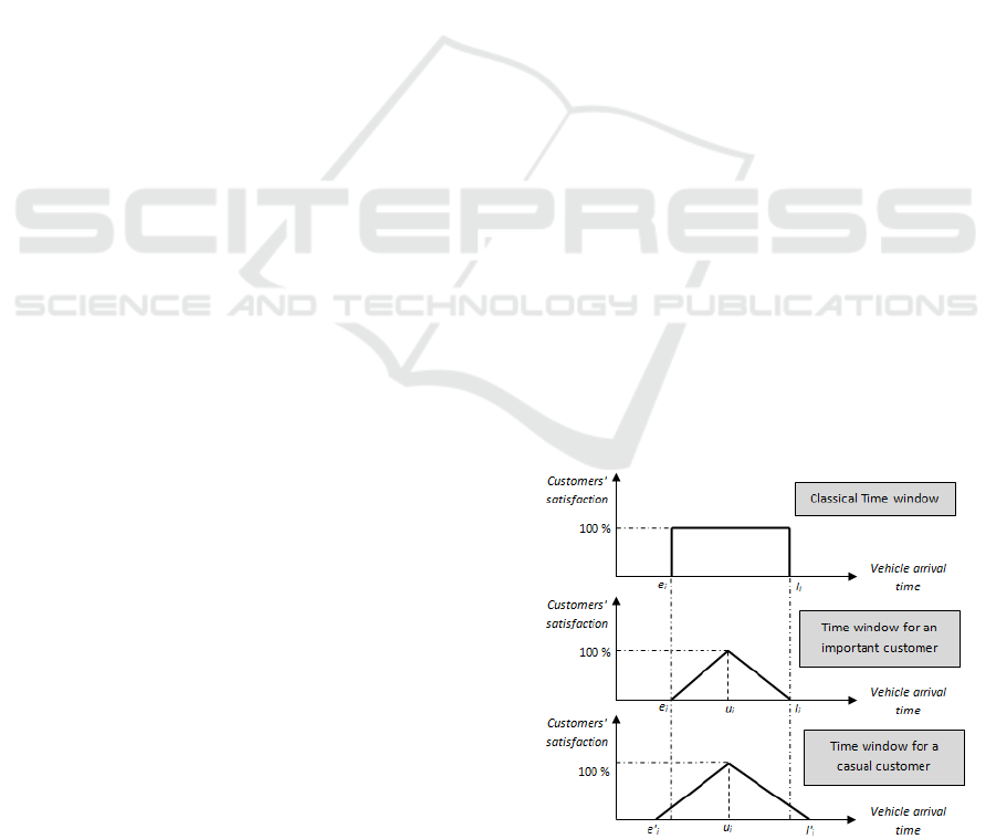
The concept of customers' satisfaction proposed
in our recent research (Ghannadpour & Hooshfar
2015) is also considered and developed here for
different kinds of customers. In this paper the
preference information of customers is represented
as a fuzzy time windows as Fig.1. In this approach,
every customers can be assigned by the expert to one
of groups (e.g., important customers (
), casual
(
) and etc.) where
∪
=\{0}.
Figure 1: Conventional and fuzzy time window for each
customer.
Multi-Objective Vehicle Routing Problem with Time Windows and Fuel Consumption Minimizing
93

According to Fig. 1, the classical time window is
changed to the triple [
,
,
] and [́
,
,
] for
important and casual customers.
(
) is the
membership function of customer i and shows the
grade of satisfaction when the start of service time is
t
i
. The start time of service for each customer i is as
=
+
where
and
are arrival and
waiting time at customer i. Therefore a new
objective function should be considered as
∑
×
(
)
∈\{}
where,
is the
importance degree of customer i.
The mathematical formulation of the proposed
model is as follows:
(4)
=
∑∑ ∑
(
×
,
+
)×
(5)
=
∑∑
(6)
=
∑
×
(
)
S.t:
(7)
∀ = 0
∑∑
≤
(8)
∀ ∈ ,
∀ ∈
∑
,
=
∑
,
≤1
(9)
∀
∈
\{0}
∑∑
,
=1
(10)
=
=
=
(
)
=
=0
(11)
∀ ∈ /{0},
∀ ∈ ,
=0
+
+
+
−(1−
) ≤
(12)
∀
∈\
{
0
}
,
∀ ≠
∈,
∀ ∈
+
+
+
−(1−
) ≤
(13)
∀ ∈
(
)
=
(
)
∗
(
1−
)
+
(
)
∗
(14)
∀ ∈
(
)
=
(
)
(
)
(
)
∗
(
1−
)
+
(
)(
)
(
)
∗
(15)
∀ ∈ \{0}
(
−(
+
)
)
∗
+
(
(
+
)−
)
∗
(
1−
)
<0
(16)
∀ ∈
≤
(
+
)
≤
(17)
∀ ∈
−≤
(
+
)
≤
+
(18)
∀ ∈ \{0}
∑∑
,
−
∑∑
,
=
(19)
∀
∈
,∀ ≠
∈
,∀ ∈
≤
×
∀,
∈,
∀ ∈
∈ {0,1},
≥0
Formulas (4-6) are the objective functions
Formula (4-5) minimize total energy consumed and
the total number of vehicles and formula (6)
maximizes the total satisfaction rates of customers.
Constraint (8) secures maximum size of fleet.
Constraints (8) and (9) define that every customer
node is visited only once by one vehicle. Constraint
(11) is the maximum travel time constraint.
Constraints (12-17) define the arrival time, and the
time windows for different kinds of customers.
Constraints (13-15) compute the satisfaction level of
each customer Constraints (13-15) are non-linear
and they have relaxed to linear constraints.
Constraint (18) indicates the load of vehicle after it
visits a customer. Constraint (19) limits the maximal
load carried by the vehicle and force
to zero
when
=0.
3 SOLUTION METHOD
This section designs an efficient evolutionary
method for tackling the proposed model that in
which objectives are met and the constraints are
satisfied. The proposed model is based on the
conventional VRPTW which is NP-hard and should
be tackled by heuristics. The evolutionary
algorithms like GA have many advantages in finding
an easy way of the solution representation and in
implementation for multi objective models and
ability of incorporation with the different operators
that improve the solutions.
ICORES 2016 - 5th International Conference on Operations Research and Enterprise Systems
94

3.1 Representation
In this method each chromosome which is a solution
to the problem, is represented by an integer string of
length . This string of customer identifiers
represents the sequence of deliveries that must be
covered by vehicles during their routes.
3.2 Pareto Ranking Procedure
The Pareto ranking procedure (Ghannadpour &
Hooshfar 2015) which tries to rank the solutions to
find the non-dominated solutions is used for
evaluation of each chromosome. In this approach,
chromosomes assigned rank 1 are non-dominated,
and inductively, those of rank i +1 are dominated by
all chromosomes of ranks 1 through i.
3.3 Population & Initialization
In this paper the method of PFIH (originally
proposed by Solomon (1987)) is used to create the
first chromosome. PFIH method defines the relation
of
=
+
+(
(
/360
)
) to find the
first customer in each new route where;
is the
distance from customer to the central depot;
is
the latest time and
is the polar coordinate angle of
the customer . Once the first customer is selected
for the current route, the heuristic selects from the
set of unrouted customers the one customer which
minimizes the total insertion cost between every
edge in the current route without violating the time
and capacity constraints.
3.4 Selection
This paper uses a standard k-tournament selection
where a tournament set of size k is randomly drawn
from the population and the chromosome with a
lower rank is selected and will then be recombined
via the recombination operators to create potential
new population.
3.5 Recombination
This paper uses the modified best cost-best rout
crossover (BCBRC), which selects a best route from
each parent and then for a given parent, the
customers in the chosen route from the opposite
parent are removed. The final step is to locate the
best possible locations for the removed customers in
the corresponding children.
3.6 Local Search
The local search (LS) is employed as mutation to the
child chromosome with a probability
. This
paper uses a -interchange mechanism as local
search method that moves customers between routes
to generate neighborhood solution for the proposed.
Given a feasible solution for the model represented
by ={
,…,
,…,
,…,
} where
is a set
of customer served by vehicle route . A -
interchange between a pair of routes
and
is a
replacement of subset
⊆
of size |
|≤ by
another subset
⊆
of size |
|≤, to get the
new route sets
,
and a new neighbouring
solution
={
,…,
,…,
,…,
} where
=
(
−
)∪
and
=(
−
)∪
. The
neighbouring
() of a given solution is the set
of all neighbors {
} generated by the λ-interchange
method for a given λ. In one version of the algorithm
called GB (global best), the whole neighborhood is
explored and the best move with lower rank is
selected. In another version, FB (first best), the first
admissible improving move is selected if exists;
otherwise the best admissible move is implemented.
In this paper 1-interchange (FB) or 2-interchange
(GB) is employed to the child chromosome with the
special probability.
4 COMPUTATIONAL ANALYSIS
In this section, since there is no any prior work on
the proposed model, a set of complete randomly
generated instances with different size (N) is
considered as numerical examples. In the first step,
the validity of new mathematical formulation for
small and medium instances are implemented by
CPLEX Solver separately (with a time limit of 2
hours) and the results are analyzed. Finally, the
quality of proposed evolutionary method is
evaluated. In this step the instances with larger size
are considered and the results obtained by the
proposed method and CPLEX Solver are analyzed.
4.1 Mathematical Modelling
Table 1 presents a summary of results obtained by
CPLEX Solver when the single objective energy
minimizing VRPTW is considered. The column
labeled “with classical cost function” gives the
findings of VRPTW when it tries to minimize the
total distance travelled by vehicles (distance
oriented); column “with new cost function” gives the
Multi-Objective Vehicle Routing Problem with Time Windows and Fuel Consumption Minimizing
95

findings of model when it tries to minimize the total
energy consumption (fuel oriented). For each
instance, the vehicles’ total traveling distance
(indicated by Dis.) and the related fuel consumption
(indicated by Related FC) are calculated when the
distance-oriented model is implemented. Moreover,
the fuel consumption (FC) and the related traveling
distance (Related Dis.) are also obtained by fuel-
oriented model. The times marked with an asterisk
show the time limit of 2 hours for the CPLEX Solver
and the solver is interrupted after this time. For some
instances there is no integer solution up to this time
limit.
It can be observed from Table 1 that for the
small/medium – scale instances, the FC obtained by
fuel oriented model is on average 5.6% lower than
the obtained by distance oriented model but with a
10.6% increase in distance traveled. In other words,
by 10.6% increase in distance traveled, the fuel cost
which is a significant part of total transportation cost
can be reduced by 5.6%. It should be noted that the
choice of any solutions (fuel & distance oriented)
depends on the DM’s preference.
Table 1: VRPTW with fuel consumption by CPLEX
Solver.
With classical cost function
N
Instance
Related FC.
CPU t.
(Sec.)
Dis.
2847.909 0.2030 115.3760 4 1
2427.428 0.2180 140.1070 5 2
4392.852 2.8750 226.6523 10 3
6106.863 13.359 303.2485 12 4
9817.879 37.765 321.6250 15 5
14827.87 7200* 497.100 20 6
-------- 7200* -------- 30 7
-------- 7200* -------- 40 8
5118.586 221.4018 Ave.
With new cost function
N
Instance
Related FC.
CPU t.
(Sec.)
Dis.
138.152 0.0541 2438.131 4 1
156.523 0.0620 2393.459 5 2
228.777 2.0150 4382.368 10 3
340.049 17.357 5933.309 12 4
376.166 69.531 9220.890 15 5
-------- 7200* -------- 20 6
-------- 7200* -------- 30 7
-------- 7200* -------- 40 8
247.9334 4873.631 Ave.
FC dev. : -5.57 / Dis dev. : 10.64 Dev. (%)
4.2 Analysis of Proposed Method
In this section, the quality of proposed evolutionary
method is evaluated. In this step the instances with
larger size are considered and the results obtained by
the proposed method and CPLEX Solver are
analyzed. The results of Mathematical Model are
found by using the weighting method as follows:
(20)
×
+
×
−
×
Where,
is the weight of objective function
estimated by DM and
∑
=1 and the objective
functions
are calculated according to relations (4-
6). The proposed heuristic is coded and run on a PC
with Core 2 Duo CPU (3.00 GHz) and 2.9 GB of
RAM. Moreover, the model is implemented under
parameters of Population size = 30 - 100, Generation
number = 500-1000, Crossover rate = 0.80, Mutation
rate = 0.40, Selection rate of improvement operators
= 0.5. It must be mentioned that the population size
and the generation number is adopted with the
problem size.
It should be noted that the Repetition of
experiments is 10 runs. Table 2 presents the average
and best values (among the non-dominated
solutions) of proposed method over 10 runs and to
the finding of CPLEX Solver.
Table 2: Average and best results over 10 experiments.
N
h−ave h−best
FC.
K
Sat.
FC
K
Sat
10 4424.69 6.0 25.20 4382.37 6 26.00
15 9845.04 6.6 33.20 9308.00 6 36.00
20 14520.1 8.1 49.50 14345.3 8 54.00
30 19150.3 12 78.40 18009.1 12 79.00
40 29308.4 16.8 103.8 25542.8 16 105.0
70 59805.0 15 117.0 50231.1 15 120.0
100 83063.7 18.6 260.5 75654.6 18 270.0
N
Deviation (%)
D
D
D
D
D
D
10 0.960 0.00 3.08 0.0 0 0
15 5.450 9.09 7.78 0.9 0 0
20 1.200 1.23 8.33 -1.6 0 0
30 5.960 0.00 0.76 --- --- ---
40 12.85 4.76 1.14 --- --- ---
70 16.01 0.00 2.50 --- --- ---
100 8.920 3.23 3.52 --- --- ---
Ave.
7.340 2.62 3.87 -0.2 0 0
ICORES 2016 - 5th International Conference on Operations Research and Enterprise Systems
96
The column labeled "ℎ−" gives the total
average findings of proposed heuristic over 10 runs
and it is divided into three columns where the each
of them represents the average of each objective
function (indicated by .
,
and
); column
"ℎ − " gives the best results of each objective
function obtained by proposed heuristic over 10
experiments (indicated by
,
and
).
Deviation between the average and best results of
proposed heuristic are listed in the columns labeled
,
and
. Moreover,
(=1,2,3)
represents the deviation between the best value of
objective function
obtained by proposed heuristic
over 10 runs and the best value found by the CPLEX
Solver. It should be noted that the listed values of
deviations represents the amount of difference
between the best and average results of proposed
method over 10 experiments and could illustrate the
consistency and reliability of results. Moreover the
deviations between the best results of proposed
method and CPLEX Solver represents the quality of
obtained results and the negative value represent the
amount of improvements obtained by the proposed
approach.
According to this table we can see the results
obtained from proposed method are rather consistent
and the average deviations over 10 experiments are
lower than 8%. Moreover, the average difference
between the best values of proposed method and
CPLEX Solver illustrates the improvement of 0.2%
in the first objective for the first three instances and
for the others the CPLEX Solver cannot find any
solution in a reasonable amount of computational
time.
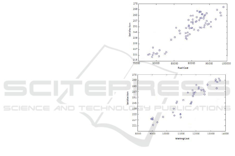
In general, the relationship between these
defined objectives is unknown until the problem is
solved in a proper multi-objective manner. These
objectives may be positively correlated with each
other or they may be conflicting to each other.
According to the results, the customers' satisfaction
rate is improved as the total fuel consumed is
deteriorated. Moreover, the waiting time imposed on
vehicles is increased in these instances due to get the
better satisfaction rate of customers. These
behaviours for the 7
th
instance of Table 6 are
illustrated in Fig.2.
The different behaviour is observed for the total
fuel consumption and the required fleets. They are
positively correlated with each other in some
instances like instance #3 and they are conflicting to
each other in others (like instance #2). By adding a
vehicle to the schedule, the load of vehicles could be
decreased along a route but the total distance
travelled by vehicles may be increased or decreased
and it is related to the geographical location and time
windows of customers [15]. So by increasing the
number of vehicles the load of vehicles is decreased
and when the distance cost of solution is changed in
the opposite direction, the total fuel consumed by
vehicles is decreased. On the other hand, in the
instance 3, although adding a vehicle provides a
schedule with a lower load of vehicles for each
route, the distance cost is much higher than that of
the basic model. Therefore the total fuel consumed
by all fleets is increased.
Figure 2: Population distribution of the 7th instance.
5 CONCLUSION
This paper presented a new model and solution for
the multi-objective vehicle routing and scheduling
problem with considering the fuel consumption rate.
Moreover, this paper considered the customers'
priority according to customer-specific time
windows, which are highly relevant to the
customers’ satisfaction level.
Besides, the proposed model was interpreted as
multi-objective optimization problem and a new
solution based on the evolutionary algorithm was
proposed. the performance on several completely
Multi-Objective Vehicle Routing Problem with Time Windows and Fuel Consumption Minimizing
97
random generated instance problems was compared
with the CPLEX Solver. The results show the
efficiency and effectively of proposed method.
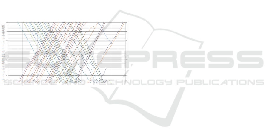
It should be noted that the proposed model is
very compatible with the constraints of reality and it
is under implementation for locomotives routing and
assignment for railway transportation division of
MAPNA Group. In this model the trains are
considered as customers and they are made up at
different stations of network and they need to
receive locomotive based on the time table of train
scheduling. Moreover, the locomotives are located at
some central depots and they depart toward the
trains to move them from their origins to their
destinations based on the train scheduling plan. One
sample of train scheduling plan is illustrated in
Fig.3. In this case, the trains with low priorities are
considered to be having the classical time windows.
Moreover, the trains with highly priority have the
fuzzy time windows and the desired time is nearest
to the earliest dispatching time of each train.
Figure 3: Typical train scheduling plan.
Moreover, the detailed schedule of each locomotive
including the departure time, trains in its
commitments, planned routes, waiting times, fuel
consumption cost and etc is corresponding to the
routes found by the proposed VRPTW and they are
identified for this route.
ACKNOWLEDGEMENTS
The authors would like to thank MAPNA Group for
its supports and financing this paper.
REFERENCES
Bektaş, T., Laporte, G., 2011. The pollution-routing
problem. Transportation Research Part B:
methodological 45: 1232-1250.
Blaseiro, S.R., Loiseau, I., Ramonet, J., 2011. An ant
colony algorithm hybridized with insertion heuristics
for the time dependent vehicle routing problem with
time windows. Computers & Operations Research 38:
954–966.
Chiang, T.C., Hsu, W.H., 2014. A knowledge-based
evolutionary algorithm for the multiobjective vehicle
routing problem with time windows. Computers &
Operations Research 45: 25-37.
Dhahri, A., Zidi, K., Ghedira, K., 2014. Variable
Neighborhood Search based Set Covering ILP Model
for the Vehicle Routing Problem with Time Windows.
Procedia Computer Science 29: 844-854.
Feng, H.M., Liao, K.L., 2014. Hybrid evolutionary fuzzy
learning scheme in the applications of traveling
salesman problems. Information Science 270: 204-
225.
Garcia-Najera, A., Bullinaria, J.A., 2011. An improved
multi-objective evolutionary algorithm for the vehicle
routing problem with time windows. Computers &
Operations Research 38: 287–300.
Garcia-Najera, A., Bullinaria, J.A., Gutiérrez-Andrade,
M.A., 2015. An evolutionary approach for multi-
objective vehicle routing problems with backhauls.
Computers & Industrial Engineering 81: 90-108.
Gaur, D.R., Mudgal, A., 2013. Singh RR. Routing
vehicles to minimize fuel consumption. Operations
Research Letters 41: 576-580.
Ghannadpour, S.F., Hooshfar, M., 2015. Multi-objective
evolutionary method for dynamic vehicle routing and
scheduling problem with customers' satisfaction level.
4st International Conference on Operations Research
and Enterprise Systems. SCITEPRESS.
Ghannadpour, S.F., Noori, S., Tavakkoli-Moghaddam, R.,
2014. A multi-objective vehicle routing and
scheduling problem with uncertainty in customers’
request and priority. Journal of Combinatorial
Optimization 28: 414-446.
Kara, I., Kara, B.Y., Yetis, M.K., 2007. Energy
Minimizing Vehicle Routing Problem. Lecture Notes
in Computer Science 4616: 62-71.
Lin, C.K.Y., 2011. A vehicle routing problem with pickup
and delivery time windows, and coordination of
transportable resources. Computers & Operations
Research 38: 1596-1609.
Mavrovouniotis, M., Yang, S., 2015. Ant algorithms with
immigrants schemes for the dynamic vehicle routing
problem. Information Science 294: 456-477.
Ombuki, B., Ross, B., Hanshar, F., 2006. Multi-Objective
Genetic Algorithm for Vehicle Routing Problem with
Time Windows. Applied Intelligence 24: 17-30.
Sivaram Kumar, V., Thansekhar, M.R., Sarvanan, R.,
Miruna Joe Amali, S., 2014. Solving multi – objective
vehicle routing problem with time windows by FAGA.
Procedia Engineering 97: 2176-2185.
Solomon, M.M., 1987. Algorithms for the vehicle routing
and scheduling problems with time window
constraints. Operations Research
35: 254–265.
Tan, K.C. Cheong, C.Y., Goh, C.K., 2007. Solving
multiobjective vehicle routing problem with stochastic
ICORES 2016 - 5th International Conference on Operations Research and Enterprise Systems
98

demand via evolutionary computation. European
Journal of Operational Research 177: 813-139.
Tan, K.C., Chew, Y.H., Lee, L.H., 2006. A hybrid
multiobjective evolutionary algorithm for solving
vehicle routing problem with time windows.
Computational Optimization and Applications 34:
115-151.
Tan, L., Lin, F., Wang, H., 2015. Adaptive comprehensive
learning bacterial foraging optimization and its
application on vehicle routing problem with time
windows. Neurocomputing 151: 1208-1215.
Tavares, G., Zsigraiova, Z., Semiao, V., Carvalho, M.G.,
2008. A case study of fuel savings through
optimisation of MSW transportation routes.
Management of Environmental Quality: An
International Journal 19: 444 – 454.
Xiao, Y., Zhao, Q., Kaku, I., Xu, Y., 2012. Development
of fuel consumption optimization model for the
capacitated vehicle routing problem. Computers &
Operations Research 39: 1419-1431.
Zhang, S., Lee, C.K.M., Choy, K.L., Ho, W., Ip, W.H.,
2014. Design and development of a hybrid artificial
bee colony algorithm for the environmental vehicle
routing problem, Transportation Research Part D:
Transport and Enviroment 31: 85-99.
Multi-Objective Vehicle Routing Problem with Time Windows and Fuel Consumption Minimizing
99
