Anomaly Detection using B-spline Control Points as Feature Space in

Annotated Trajectory Data from the Maritime Domain

Mathias Anneken

, Yvonne Fischer

and J

urgen Beyerer

1,2

Fraunhofer Institute of Optronics, System Technologies and Image Exploitation (Fraunhofer IOSB), Karlsruhe, Germany

Vision and Fusion Laboratory, Karlsruhe Institute of Technology (KIT), Karlsruhe, Germany

Keywords:

B-spline Interpolation, Support Vector Machines, Artiﬁcial Neural Networks, Multilayer Perceptron, Gaussian

Mixture Models, Anomaly Detection, Trajectories, Maritime Domain.

Abstract:

The detection of anomalies and outliers is an important task for surveillance applications as it supports oper-

ators in their decision making process. One major challenge for the operators is to keep focus and not to be

overwhelmed by the amount of information supplied by different sensor systems. Therefore, helping an op-

erator to identify important details in the incoming data stream is one possibility to strengthen their situation

awareness. In order to achieve this aim, the operator needs a detection system with high accuracy and low

false alarm rates, because only then the system can be trusted. Thus, a fast and reliable detection system based

on b-spline representation is introduced. Each trajectory is estimated by its cubic b-spline representation. The

normal behavior is then learned by different machine learning algorithm like support vector machines and

artiﬁcial neural networks, and evaluated by using an annotated real dataset from the maritime domain. The

results are compared to other algorithms.

1 INTRODUCTION

As technology progresses, the amount of sensors and

their recorded data in surveillance applications in-

creases. Therefore, operators of such systems need

to be supported to maintain an overview about all im-

portant object movements and their impact. In order

to help the operators, anomaly detection systems are

introduced into the surveillance systems. The aim is

to identify patterns that reveal an unexpected behavior

of objects, which signiﬁcantly differs from normal be-

havior prior recorded or modeled by domain experts.

For an operator to accept the assistance of such

a system, it must be reliable. This means in partic-

ular, that the system must be able to classify the be-

havior with a low false alarm rate and high accuracy.

Else, the operator loses his faith in the system and

might start to ignore it. Another important aspect is

the method of displaying the unusual behavior. Only

if the operator is able to clearly identify the reason for

the alarm, he will be able to take the correct further

steps.

Therefore, an algorithm with high precision and

recall is introduced. First, related work regarding the

anomaly detection, the algorithm and the application

domain (here, the maritime domain) is described. Af-

terwards, the main idea of the algorithm is explained

and an empirical evaluation with annotated real tra-

jectory data is conducted. At the end, a conclusion

and insight into future work are given.

2 RELATED WORK

The overview of general anomaly detection algo-

rithms by Chandola et al. (2009) gives a ﬁrst im-

pression about the versatility of different approaches

and domains of outlier and novelty detection algo-

rithms. The ﬁeld ranges from surveillance applica-

tion to computer security and fraud detection. Morris

and Trivedi (2008) give an overview about anomaly

detection specially by using optical sensors. They

divide the surveyed works into different applications

like trafﬁc surveillance and interactions between mul-

tiple objects, and cluster these works by the used tech-

niques and the method of information retrieval from

the optical inputs.

The idea of the proposed algorithm is to reduce the

complexity of a trajectory by using b-splines. Similar

to this approach, Naftel and Khalid (2006) use poly-

nomials and other functions to approximate the trajec-

tories, while assuming normal distribution in the co-

250

Anneken, M., Fischer, Y. and Beyerer, J.

Anomaly Detection using B-spline Control Points as Feature Space in Annotated Trajectory Data from the Maritime Domain.

DOI: 10.5220/0005655302500257

In Proceedings of the 8th International Conference on Agents and Artiﬁcial Intelligence (ICAART 2016) - Volume 2, pages 250-257

ISBN: 978-989-758-172-4

efﬁcient feature space for the clusters. Further, they

propose a Mahalanobis classiﬁer to detect anomalies

in the data. A self-organizing map is used to estimate

the similarities between trajectories. The algorithm is

validated by using different datasets, i.e. identiﬁca-

tion of sign language and video surveillance footage.

Melo et al. (2006) propose a feature space using

low-degree polynomials for the detection and classiﬁ-

cation of road lanes. For the clustering of similar tra-

jectories a K-Means algorithm is used. The different

lanes are further classiﬁed into different categories.

The proposed algorithm is tested with real data.

Dahlbom and Niklasson (2007) use splines to rep-

resent the main trajectory of a cluster. Therefore, the

underlying data is clustered using the mean of the nor-

malized distances between each trajectory point and

its nearest cluster point. Afterwards, the clusters are

estimated by using splines in order to reduce the com-

plexity of the representation.

Especially in the maritime domain, anomaly de-

tection is an active ﬁeld of research in itself, e.g.,

de Vries and van Someren (2012) use piecewise lin-

ear segmentation methods to compress trajectories of

maritime vessels. These compressed trajectories are

then clustered and anomaly detection is performed by

using kernel methods. Furthermore, expert domain

knowledge is incorporated. The algorithms are vali-

dated with a dataset from the Netherlands’ coast near

Rotterdam.

An algorithm that estimates a mean path for nor-

mal routes is proposed by Rosen and Medvedev

(2012). The mean path is deﬁned as the trajectory

which minimizes the euclidean distance to every other

trajectory in the same cluster. Anomalies are then de-

tected by comparing a new trajectory with this mean

path and an anomaly score is calculated. The algo-

rithm is evaluated by using simulated data as well as

a real dataset.

Guillarme and Lerouvreur (2013) propose an un-

supervised algorithm for modeling routes by using

data from a satellite based Automatic Identiﬁcation

System (AIS). First, the recorded trajectories are par-

titioned by using a stops and moves of trajectories al-

gorithm. The move parts of the trajectories are further

divided by using a piecewise linear segmentation or a

sliding window approach. This results in segments of

similar movement. These segments are clustered us-

ing the OPTICS algorithm. Afterwards, hand-picked

clusters are used for modeling the vessels’ motion-

patterns. First results for this algorithm using real data

are illustrated in the paper.

Shao et al. (2014) use a fuzzy k-nearest neighbors

and fuzzy c-means approach to conduct trajectory

correlation and clustering. Therefore, fuzzy logic is

utilized to model uncertainties in the tracks. The pro-

posed algorithms are evaluated using different types

of sensing systems.

Fischer et al. (2014) present a method to model

speciﬁc situations based on dynamic Bayesian net-

works. The main idea is to utilize expert knowledge

to describe situations of interest. For the evaluation

a speciﬁc situation, namely an incoming suspicious

smuggling vessel, is modeled and the results for dif-

ferent parameters are shown. The described situation

is translated from a situational dependency network

to a dynamic Bayesian network. Therefore, several

parameters must be chosen. Fischer et al. present a

possible approach to automatically specify these pa-

rameters.

3 ALGORITHM

A trajectory recorded by a surveillance system cannot

easily be compared to another due to

• different lengths,

• different sample rates, and

• different numbers of points.

In order to compare different trajectories several ap-

proaches are possible. E.g., dynamic time warping

is used by Vakanski et al. (2012) to learn trajectories

demonstrated by human in order to program a robot.

Laxhammar and Falkman (2011) use the Hausdorff

metric to compare two trajectories. Here, a trajectory

will be represented in a way, that its complexity will

be reduced and direct comparison between itself and

other trajectories will be possible.

A trajectory has a speciﬁc length n and consists of

multiple points p

= (p

i,lon

, p

i,lat

)

with i = 1, . . . , n,

where p

i,lon

is the longitude and p

i,lat

is the latitude

position of the i-th point. Therefore, a trajectory t is

given by t = {p

| i = 1, . . . , n}. The idea is now to

reduce the number of points, in such a way, that the

resulting trajectory can be compared by using e.g. the

euclidean distance.

Therefore, the trajectory is estimated by using a

b-spline representation. A b-spline interpolation con-

nects several (cubic) functions to interpolate a given

set of points. To assess a new trajectory, it has to be

compared with recorded normal trajectories. Hence,

a normal model of the trajectory in the observed area

will be generated by using machine learning algo-

rithms.

Anomaly Detection using B-spline Control Points as Feature Space in Annotated Trajectory Data from the Maritime Domain

251

3.1 B-spline Interpolation

In order to estimate the b-spline representation of

a trajectory, the FORTRAN routine parcur from the

FITPACK is used with the Python bindings provided

by SciPy (Jones et al., 2001). The estimated b-

spline consists of cubic functions with a prior de-

ﬁned amount of sections. Thus, each trajectory has

the same amount of control points. Each b-spline

is deﬁned by its control points. Therefore, a trajec-

tory with n points is reduced to the number of con-

trol points n

resulting in a feature space of dimension

2 · n

The resulting control points are used as feature

vector to train the machine learning algorithms. Em-

pirical investigation have shown, that for the used

dataset 4 control points are enough to represent the

trajectories. Therefore, the feature space is set to

x = (c

, c

)

(1)

with the control point

= (c

i,lon

, c

i,lat

)

, i = 1, . . . , 4. (2)

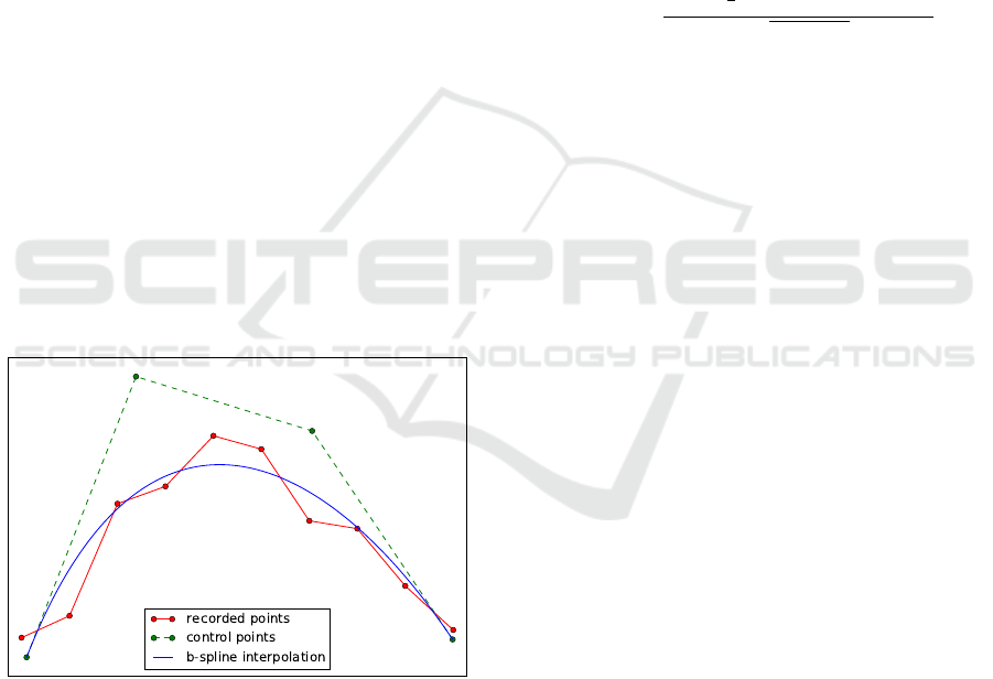
Figure 1 shows an example for a spline interpo-

lation. The red line and dots are the recorded data.

The idea is now to ﬁnd a spline, representing the line.

Therefore, the SciPy algorithms is used, to estimate

the control points for the given input data. The re-

sults are the green control points and the interpolated

blue line. As described by Gallier (1999), a spline is

uniquely determined by its control points.

Figure 1: Example spline with control points.

3.2 Machine Learning Methods

The control points as feature vector are used to train

different machine learning algorithms:

• Gaussian Mixture Models (GMM),

• Support Vector Machines (SVM), and

• Artiﬁcial Neural Networks (ANN) in form of

feedforward Multilayer Perceptrons (MLP)

3.2.1 Gaussian Mixture Models

A GMM estimates the underlying probability den-

sity function of the data by using an expectation-

maximization (EM) algorithm. It consists of the sum

of n normal distributions with the mean vector µ

the dimension k and the covariance matrix Σ

for each

component given by the parameter set θ

= {Σ

, µ

The whole probability density function is then given

f (x) =

∑

i=1

(x, θ

) (3)

with the normal distribution for each component

given by

(x, θ

) =

exp



−

(x − µ

)

−1

(x − µ

)



(2π)

|Σ

. (4)

The GMM and the EM-algorithm are implemented

in the scikit-learn machine learning framework for

Python (Pedregosa et al., 2011).

A GMM is learned unsupervised. Thus, no la-

bels are necessary, but the algorithms will not yield

an anomaly as a speciﬁc class. Therefore in order to

detect an anomaly, a threshold g

min

is set. If the eval-

uated log-likelihood of a new trajectory is below this

threshold, the trajectory will be marked as anomaly.

Anomalies are deﬁned as occurring only sparsely;

therefore, the threshold will be estimated by using

a speciﬁc percentile of the trained log-likelihood re-

sults. Here, this kind of learning algorithm is called

unsup-GMM.

Additionally as another approach, the GMM is

trained by using only the normal trajectories. The

threshold is then chosen as the lowest log-likelihood

predicted for the training data. This algorithm will

be identiﬁed as sup-GMM. Further information on

GMMs and the learning algorithm is, e.g., given by

Barber (2014).

3.2.2 Support Vector Machines

A SVM used as a classiﬁer will divide a set of objects

into classes. Therefore, the border in the feature space

between the classes should be optimized, i.e. the mar-

gin between the border and each object in the train-

ing set should be as large as possible. In general, the

classes need to be linear separable by a hyperplane,

while the feature space may be of high dimensional-

ity. To counter this problem, different kernels can be

used for the SVM. Here, a radial basis function with

the parameter γ is used. Furthermore, a penalty pa-

rameter C is available for optimizing the results of the

classiﬁer.

ICAART 2016 - 8th International Conference on Agents and Artiﬁcial Intelligence

252

The parameter C balances between a simple and

smooth decision surface and the misclassiﬁcation of

training examples, i.e., a low C results in a smooth

surface a high C in mostly correctly classiﬁed exam-

ples. The inﬂuence of a single data point of the train-

ing set is regulated by the parameter γ. A high value

for γ means, that training examples need to be close

to each other to affect each other.

These parameters are chosen by using a grid

search. Further details on SVMs are, e.g., available

by Kung (2014). The implementation provided by

the framework scikit-learn (Pedregosa et al., 2011) is

used.

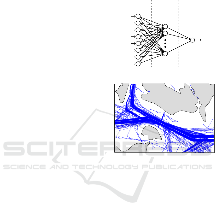
3.2.3 Multilayer Perceptron

As a non-deterministic machine learning method, a

multilayer perceptron with a truncated Newton algo-

rithm for the backpropagation based training provided

by the implementation FFNET framework for Python

(Wojciechowski, 2011) is used. The neural network

consists of 3 layers, one input, one output and one

hidden layer. As input, the control points are used.

The output is the label normal or anomaly. The layers

are connected as seen in Figure 2. The hidden layer

consists of n

units.

As activation function the input layer uses the

identity function, whereas all other units use a sig-

moid activation function. Due to its non-deterministic

nature, the training is performed several times and the

best model is used. Further details on ANN are, e.g.,

available by Shalev-Shwartz and Ben-David (2014).

3.2.4 Estimation of Optimal Parameters

For all algorithms, the optimal parameters are esti-

mated by using a grid search with a 10-fold cross-

validation. For the GMM the number of components

n and the threshold g

min

, for the SVM the parameters

C and γ, and for the MLP the number of units in the

hidden layer n

are estimated.

4 EMPIRICAL EVALUATION

In order to validate the algorithm, an annotated real

dataset from the maritime domain is used. First, the

dataset and the test setup are explained. Afterwards,

the results for the different algorithms are given.

4.1 Dataset and Test Setup

As dataset for the evaluation, real ship trafﬁc between

Lolland and Fehmarn in the Baltic Sea is chosen. The

4,lon

4,lat

3,lon

3,lat

2,lon

2,lat

1,lon

1,lat

input

layer

hidden

layer

output

layer

out

Figure 2: Structure of the feedforward MLP used for the

training.

Figure 3: Whole dataset of tanker and cargo vessels be-

tween Lolland in the north and Fehmarn and the German

mainland in the south. The grey polygons are landmasses,

the blue lines represent the vessel trafﬁc.

tracks were recorded in a period of 7 days using the

AIS system. For the validation, only the data of the

tanker and cargo vessels is used, as these types have

a similar behavior. All 758 unique tracks (191 tracks

by tankers and 567 by cargo vessels) can be seen in

Figure 3. The dataset is annotated, i.e. each point in

the dataset is either marked as normal or as abnormal.

Therefore, the ground truth is given for calculating the

precision and recall for all algorithms.

For the evaluation a 10-fold stratiﬁed cross-vali-

dation is used. This means, that the whole dataset is

divided into 10 folds and each of the folds contains

the same ratio of abnormal trajectories as labeled in

the whole dataset. As described by Witten and Frank

(2005), a 10-fold cross-validation has shown to yield

the best estimate of error. Therefore, the results gen-

erated by the different folds is averaged. The whole

cross-validation is performed 10 times and these re-

sults are averaged in order to get a reliable error esti-

mate.

The results are compared to algorithms used by

Laxhammar et al. (2009). In their investigation a

Anomaly Detection using B-spline Control Points as Feature Space in Annotated Trajectory Data from the Maritime Domain

253

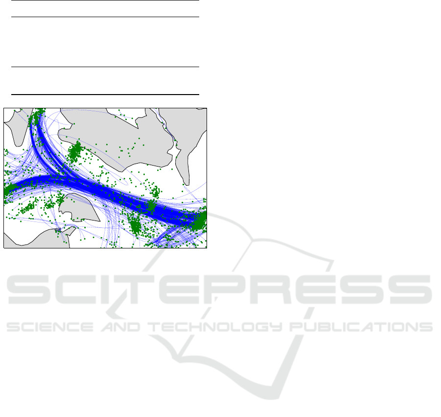
Table 1: Optimal parameters for the evaluation.

Algorithm Parameters

unsup-GMM n = 6; g

min

= 35th percentile

sup-GMM n = 30

SVM C = 10000; γ = 0.1

MLP n

= 25

L-GMM n = 75; grid: 5x5

KDE h = 0.06

Figure 4: B-spline representations of all trajectories in the

dataset. The blue lines represent the splines, the green dots

represent the control points.

GMM (here named L-GMM) and a Kernel Density

Estimation (KDE) are compared for their ability to

detect anomalies in sea trafﬁc. These algorithms are

used to determine the underlying probability density

function representing the distribution of data points.

Therefore, these algorithms can assess each incoming

data point on its own.

As described by Anneken et al. (2015) in their

quantitative evaluation, the algorithms are trained

with normal data only, which yields a better result for

the overall f1-score as well as for the single precision

and recall scores. For the GMM, the area is divided

by a grid and for each cell in the grid, the anomaly

detection is performed separately. For the KDE, the

bandwidth h has to be chosen. A bandwidth chosen

too high will result in underﬁtting and too low in over-

ﬁtting.

For all algorithms, the optimal parameters are cho-

sen by using a grid search. The resulting optimal pa-

rameters are shown in Table 1.

4.2 Results

In Figure 4, the b-spline representations for all trajec-

tories are shown. Each blue line represents one tra-

jectory. For the estimation to work properly, the raw

trajectories need to contain at least 4 points. For some

transformed trajectories, the course can now be seen

to run over islands. This is a result of using only a lim-

ited amount of control points. The resulting trajecto-

ries are smoothed; therefore, the exact course is lost.

The control points for each trajectory are depicted by

green dots. The ﬁrst and last point indicate the be-

ginning and the end of the trajectory. Thus, there are

clusters of green dots at the border of the ﬁgure. Fur-

thermore, several other clusters of green dots can be

seen in the image.

The averaged precision, recall and f1-score for the

whole dataset for the b-spline feature approaches as

well as the point-based approaches is shown in Table

2. These scores are given regarding the detection of

anomalies and not the representation of normal data,

i.e. a correctly detected anomaly is a true positive,

whereas normal data marked as normal data is a true

negative. Furthermore, the ground truth and the re-

sults for one test fold using the different learning al-

gorithms for the b-spline representation is depicted in

Figure 5. The blue trajectories are detected as normal,

whereas the red ones are detected as anomalies.

Each sub-ﬁgure in Figure 5 underlines the scores

given in Table 2. The SVM-based and MLP-based

algorithms yield better results than the unsup-GMM

and the sup-GMM. Most anomalies are detected cor-

rectly by the SVM and MLP approach, only a few

are not found and some are detected as anomaly even

though they are not.

The f1-scores for the unsup-GMM is the low-

est for the b-spline feature approaches, followed by

the sup-GMM (12.4% higher), the SVM (16.9%

higher), and the MLP with the highest f1-score

(23.8% higher). The precision and recall differ sig-

niﬁcantly for both GMM approaches. This can also

be seen in Figure 5(b) and Figure 5(c). Here, the

sup-GMM is able to identify the anomalies which

are quite far away from the normal trajectories, but

nearly no abnormal trajectory near the normal ones

is marked as anomaly. Therefore, nearly all detected

anomalies are true positives.

Comparing the b-spline feature methods with the

L-GMM and the KDE approach, it is evident, that

even the unsup-GMM with the worst results is able to

outperform the point-based approaches. The f1-score

for the unsup-GMM is 30.5% higher than the one for

the L-GMM and 18.7% higher than the one for the

KDE. Comparing the MLP approach to the L-GMM,

the MLP’s f1-score is even 61.6% higher than the one

for the L-GMM.

Furthermore, the false positive rate (FP rate) is

given for each algorithm in Table 2. The best FP rate

is achieved with the b-spline approach using a SVM

and a MLP, and the L-GMM. By far the unsup-GMM

ICAART 2016 - 8th International Conference on Agents and Artiﬁcial Intelligence

254

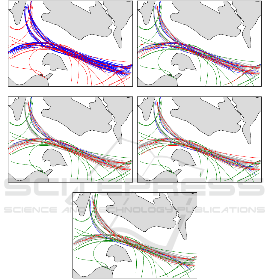
(a) Ground truth (b) unsup-GMM

(e) MLP

Figure 5: The results for tanker and cargo vessels for one fold. In Figure 5(a), the blue lines are marked as normal trajectories,

whereas the red ones are detected as anomalies. For all other sub-ﬁgures, anomalies detected as anomalies are depicted

with green lines, anomalies detected as normal with red lines, normal trajectories detected as anomalies with blue lines, and

normal trajectories detected as normal with grey lines. The grey polygons are landmasses (in the north Lolland and other

Danish islands and in the south Fehmarn and the German mainland), the white background is the Baltic Sea.

has the worst FP rate of the tested algorithms. This

is a result of using all the available data (normal and

abnormal) as training data. The sup-GMM has a FP

rate in between the L-GMM and the KDE.

The results of the unsup-GMM and the sup-GMM

are far worse than the ones for the SVM and the MLP.

The precision for the unsup-GMM is lower than the

one for the sup-GMM, SVM, and MLP, whereas the

recall is as high as the one for the SVM. The preci-

sion for the sup-GMM is 3.9% lower than the SVM

one, but the recall is the lowest of the b-spline fea-

ture methods. For the unsup-GMM, the problem is

founded in the usage of all available training data dur-

ing the learning phase. Even abnormal data is used

Anomaly Detection using B-spline Control Points as Feature Space in Annotated Trajectory Data from the Maritime Domain

255

Table 2: Averaged results of the anomaly detection for tanker and cargo vessels.

Score

B-spline features Laxhammar et al. (2009)

unsup-GMM sup-GMM SVM MLP L-GMM KDE

precision 0.6793 0.8923 0.9282 0.9398 0.6547 0.6250

recall 0.7650 0.7401 0.7692 0.8468 0.4763 0.5883

FP rate 0.1643 0.0407 0.0271 0.0248 0.0256 0.0545

f1-score 0.7196 0.8090 0.8412 0.8908 0.5514 0.6061

for learning the underlying distribution, resulting in

lower precision and recall. Comparing the unsup-

GMM results in Figure 5(b) with the ground truth in

Figure 5(a), the false classiﬁcation of normal and ab-

normal data can be seen. Several trajectory labeled as

normal are classiﬁed as anomaly and vice versa.

Comparing Figure 5(d) and Figure 5(e) with each

other, the difference is not that signiﬁcant. There are

some occasions, where the MLP classiﬁes the data

differently than the SVM, resulting in a better over-

all classiﬁcation for the MLP (the f1-score is 5.9%

higher for the MLP than for the SVM).

5 CONCLUSIONS

Depending on the machine learning methods, the pro-

posed algorithm has a high precision and recall score.

The introduced algorithm, especially based on the

MLP, outperforms the algorithms used by Laxham-

mar et al. (2009) by far.

Nevertheless, the algorithm has some drawbacks.

First, due to the smoothing of the trajectories, small

anomalies cannot be detected by this approach. Sec-

ond, the whole trajectory must be known to use this

algorithms for anomaly detection. Therefore, it can

only be used for post-processing, or in case that the

execution time for each trajectory is rather short and

therefore the assessment will be available near real-

time. Third, the whole trajectory may not be too com-

plicated. This is also a result of the smoothing, as

the estimation for long and complicated trajectories is

rather bad.

6 FUTURE WORK

To improve the shown drawbacks, several solutions

are plausible. In order to make the algorithm usable

for real-time analysis, the possible endpoint of a tra-

jectory can be estimated and by using this estimation,

a b-spline representation can be predicted.

Furthermore, the trajectories can be segmented,

e.g., by dividing the trajectories at turns. These seg-

ments can be used to build a Markov Chain or simi-

lar to represent the transition between the segments.

This will tackle two problems at once. First, smaller

anomalies might be detectable, as the trajectories are

shorter and therefore the smoothing has less impact.

Second, a real-time prediction for vessels is possible,

as for each vessel a path can be predicted and thus

anomalies can be detected earlier.

ACKNOWLEDGEMENTS

The underlying projects to this article are funded by

the WTD 81 of the German Federal Ministry of De-

fense. The authors are responsible for the content of

this article.

REFERENCES

Anneken, M., Fischer, Y., and Beyerer, J. (2015). Evalua-

tion and comparison of anomaly detection algorithms

in annotated datasets from the maritime domain. In

SAI Intelligent Systems Conference 2015.

Barber, D. (2014). Bayesian Reasoning and Machine

Learning. Cambridge University Press.

Chandola, V., Banerjee, A., and Kumar, V. (2009).

Anomaly detection: A survey. ACM Computing Sur-

veys, 41(3):15:1–15:58.

Dahlbom, A. and Niklasson, L. (2007). Trajectory cluster-

ing for coastal surveillance. In Information Fusion,

2007 10th International Conference on, pages 1–8.

de Vries, G. K. D. and van Someren, M. (2012). Ma-

chine learning for vessel trajectories using compres-

sion, alignments and domain knowledge. Expert Sys-

tems with Applications, 39(18):13426 – 13439.

Fischer, Y., Reiswich, A., and Beyerer, J. (2014). Model-

ing and recognizing situations of interest in surveil-

lance applications. In Cognitive Methods in Situation

Awareness and Decision Support (CogSIMA), 2014

IEEE International Inter-Disciplinary Conference on,

pages 209–215.

Gallier, J. (1999). Curves and Surfaces in Geometric Mod-

eling: Theory and Algorithms. Morgan Kaufmann.

Guillarme, N. L. and Lerouvreur, X. (2013). Unsupervised

extraction of knowledge from s-ais data for maritime

ICAART 2016 - 8th International Conference on Agents and Artiﬁcial Intelligence

256

situational awareness. In 16th International Confer-

ence on Information Fusion Istanbul, Turkey, July 9-

12, 2013.

Jones, E., Oliphant, T., Peterson, P., et al. (2001). SciPy:

Open source scientiﬁc tools for Python. [Online;

http://www.scipy.org/; accessed 2015-09-01].

Kung, S. Y. (2014). Kernel Methods and Machine Learning.

Cambridge University Press.

Laxhammar, R. and Falkman, G. (2011). Sequential confor-

mal anomaly detection in trajectories based on haus-

dorff distance. In Information Fusion (FUSION),

2011 14th International Conference on, pages 1–8.

Laxhammar, R., Falkman, G., and Sviestins, E. (2009).

Anomaly detection in sea trafﬁc - a comparison of the

gaussian mixture model and the kernel density. In 12th

International Conference on Information Fusion Seat-

tle, WA, USA, July 6-9, 2009.

Melo, J., Naftel, A., Bernardino, A., and Santos-Victor, J.

(2006). Detection and classiﬁcation of highway lanes

using vehicle motion trajectories. Intelligent Trans-

portation Systems, IEEE Transactions on, 7(2):188–

200.

Morris, B. and Trivedi, M. (2008). A survey of vision-based

trajectory learning and analysis for surveillance. Cir-

cuits and Systems for Video Technology, IEEE Trans-

actions on, 18(8):1114–1127.

Naftel, A. and Khalid, S. (2006). Classifying spatiotem-

poral object trajectories using unsupervised learning

in the coefﬁcient feature space. Multimedia Systems,

12(3):227–238.

Pedregosa, F., Varoquaux, G., Gramfort, A., Michel, V.,

Thirion, B., Grisel, O., Blondel, M., Prettenhofer,

P., Weiss, R., Dubourg, V., Vanderplas, J., Passos,

A., Cournapeau, D., Brucher, M., Perrot, M., and

Duchesnay, E. (2011). Scikit-learn: Machine learning

in Python. Journal of Machine Learning Research,

12:2825–2830.

Rosen, O. and Medvedev, A. (2012). An on-line algorithm

for anomaly detection in trajectory data. In American

Control Conference (ACC), 2012, pages 1117–1122.

Shalev-Shwartz, S. and Ben-David, S. (2014). Understand-

ing Machine Learning - From Theory to Algorithms.

Cambridge University Press.

Shao, H., Japkowicz, N., Abielmona, R., and Falcon, R.

(2014). Vessel track correlation and association using

fuzzy logic and echo state networks. In Evolutionary

Computation (CEC) 2014, IEEE Conference on.

Vakanski, A., Mantegh, I., Irish, A., and Janabi-Shariﬁ,

F. (2012). Trajectory learning for robot program-

ming by demonstration using hidden markov model

and dynamic time warping. Systems, Man, and Cy-

bernetics, Part B: Cybernetics, IEEE Transactions on,

42(4):1039–1052.

Witten, I. H. and Frank, E. (2005). Data Minig: Practi-

cal Machine Learning Tools and Techniques with Java

Implementations. Morgan Kaufmann Publishers, 2

edition.

Wojciechowski, M. (2011). Feed-forward neural network

for python. [online; http://ffnet.sourceforge.net/; ac-

cessed 2015-09-01].

Anomaly Detection using B-spline Control Points as Feature Space in Annotated Trajectory Data from the Maritime Domain

257