Similarity Function Learning with Data Uncertainty
Julien Bohn
´
e
1,2
, Sylvain Colin
1
, St
´
ephane Gentric
1
and Massimiliano Pontil
2
1
Safran Morpho, Issy-les-Moulineaux, France
2
University College London, Department of Computer Science, London, U.K.
Keywords:
Similarity Function, Uncertain Data, Missing Data, Face Recognition.
Abstract:
Similarity functions are at the core of many pattern recognition applications. Standard approaches use fea-
ture vectors extracted from a pair of images to compute their degree of similarity. Often feature vectors are
noisy and a direct application of standard similarly learning methods may result in unsatisfactory performance.
However, information on statistical properties of the feature extraction process may be available, such as the
covariance matrix of the observation noise. In this paper, we present a method which exploits this information
to improve the process of learning a similarity function. Our approach is composed of an unsupervised dimen-
sionality reduction stage and the similarity function itself. Uncertainty is taken into account throughout the
whole processing pipeline during both training and testing. Our method is based on probabilistic models of
the data and we propose EM algorithms to estimate their parameters. In experiments we show that the use of
uncertainty significantly outperform other standard similarity function learning methods on challenging tasks.
1 INTRODUCTION
Many computer vision tasks like face verification or
k-nearest neighbors classification include two steps:
a feature extraction step which transforms the image
into a feature vector and the computation of similar-
ity scores between the feature vectors. The similarity
score is the output of a parametric similarity function
which is learned from training data.
The quality of extracted features has a strong in-
fluence on the system’s overall performance and, in
many applications, the uncertainty of a specific fea-
ture varies from one image to another. For example,
the uncertainty of a local feature describing the top
left corner of an image could depend on the signal to
noise ratio in that area which can be different from
one image to another and independent of the signal to
noise ratio in, say, the bottom right corner. Nonethe-
less, this uncertainty information is ignored by most
machine learning algorithms which simply treat each
sample as a point in the feature space. To overcome
this limitation, uncertainty-aware methods consider
each sample as a probability distribution which is pro-
vided by the feature extraction process. Each sample
has a specific distribution which reflects the uncer-
tainty in the corresponding features.
In this paper, we design a method which takes ad-
vantage of uncertainty information to build a better
similarity function and we show that it helps to cope
with images of different resolutions, pose variation or
occlusion. Specifically, we extend the Joint Bayesian
method (Chen et al., 2012) to deal with uncertainty in-
formation. The Joint Bayesian method is a similarity
function learning algorithm which has been success-
fully applied to face verification. On the challenging
LFW dataset (Huang et al., 2007) it is used in several
of the best performing methods: (Cao et al., 2013),
(Chen et al., 2012), (Sun et al., 2014a) and (Sun et al.,
2014b).
This paper is organized as follows. In Section 2
we discuss the related work. To take into account
uncertainty throughout the whole processing pipeline
we propose an uncertainty-aware dimensionality re-
duction algorithm and a similarity function that we
describe respectively in Section 3 and 4. Section 5
presents experiments which indicate the advantage of
using uncertainty and finally we summarize our find-
ings in Section 6.
2 RELATED WORK
Similarity learning has been a popular topic both in
the machine learning and computer vision commu-
nities. Many methods have been developed in the
recent years. Some are designed to improve near-
Bohné, J., Colin, S., Gentric, S. and Pontil, M.
Similarity Function Learning with Data Uncertainty.
DOI: 10.5220/0005648601310140
In Proceedings of the 5th International Conference on Pattern Recognition Applications and Methods (ICPRAM 2016), pages 131-140
ISBN: 978-989-758-173-1
Copyright
c
 2016 by SCITEPRESS – Science and Technology Publications, Lda. All rights reserved
131

est neighbors classification like LMNN (Weinberger
and Saul, 2009), whereas others such as ITML (Davis
et al., 2007) or LDML (Guillaumin et al., 2009) are
more generic. Several methods assume a statistical
model of the data, often based on normal distribu-
tions, to build the similarity function. For example,
the Linear Discriminant Analysis (LDA) or more re-
cent methods like the Probabilitic LDA (Prince and
Elder, 2007), KISSME (K
¨
ostinger et al., 2012) or
the Joint Bayesian method (Chen et al., 2012) are all
based on Gaussian models. As opposed to most sim-
ilarity function methods, the Joint Bayesian method
does not operate in the space formed by the difference
of feature vectors but works on the joint distribution
of feature vectors pair. To deal with uncertain data,
this paper proposes to generalize the Joint Bayesian
method by considering each sample as a probability
distribution in the feature space instead of a simple
point.
Whereas, up to our knowledge, this kind of ap-
proach has never been applied to similarity function
learning, this idea has been explored for other ma-
chine learning tasks. Several classification algorithms
have been extended to deal with uncertain data such as
SVM (Bi and Zhang, 2004) and (Shivaswamy et al.,
2006), decision trees (Tsang et al., 2011), or naive
Bayes classifier (Ren et al., 2009). Clustering al-
gorithms have also been adapted to uncertain data,
see, for example, (Cormode and McGregor, 2008),
(Kriegel and Pfeifle, 2005) and references therein.
The Probabilistic PCA (PPCA) (Tipping and
Bishop, 1999) gives a probabilistic view point of the
standard PCA. We have been inspired by it to design
our dimensionality reduction algorithm presented in
the next section.
3 DIMENSIONALITY
REDUCTION
In computer vision and in face recognition in partic-
ular, raw features extracted from images (LBP, SIFT,
Gabor jets, etc.) are often very high dimensional so,
in order to limit the computational cost, most similar-
ity function methods start with a dimensionality re-
duction step. PCA has been shown to be both sim-
ple and effective for this task but does not take into
account any uncertainty information. In the next sec-
tion, we propose a dimensionality reduction method
which uses the uncertainty information to learn the
low dimensional space and to project new feature vec-
tors into it.
3.1 Uncertainty-aware Probabilistic
PCA
Our dimensionality reduction method, Uncertainty-
Aware Probabilistic PCA (UA-PPCA), uses a gener-
ative model similar to that used in Probabilistic PCA
(Tipping and Bishop, 1999) or Factor Analysis. This
latent variable model explains the observation
e
x as the
sum of a linear transformation of a low dimensional
latent variable x and some noise. x is assumed to
follow the standard multivariate normal distribution
N (0,I). Specifically, our model can be written as
e
x = µ +W x +
e
ε
x
(1)
where
e
x ∈ R
n
, µ ∈ R
n
is the center of the observation
space, W ∈ R
n×m
relates the observation and the la-
tent space, x ∈ R
m
and
e
ε
x
∈ R
n
is a Gaussian noise
of distribution N (0,
e
S
x
). The uncertainty associated
with the feature vector
e
x is represented by the covari-
ance matrix
e
S
x
.
The difference between PPCA or Factor Analysis
and our method is that we make a different assump-
tion on the noise distribution. In PPCA and Factor
Analysis, a single covariance matrix for the noise is
common to all samples. This makes possible to learn
this matrix from the data. In contrast, in UA-PPCA,
each vector
e
ε
x
has its own covariance matrix
e
S
x
which
reflects the uncertainty in each component of the spe-
cific feature vector
e
x. The matrices
e
S
x
being all differ-
ent, they cannot be learned and therefore have to be
provided by the feature extractor. They are regarded
as fixed during the learning process.
Considering that two features are uncorrelated is
very different from saying that the noises which af-
fect them are uncorrelated. In a picture of a face, the
appearance of the two eye are obviously correlated.
However, the noises affecting them on a given image
can very well be different if, let say, there is a cast
shadow on one side of the face. In this paper, we as-
sume that the noise is uncorrelated and therefore con-
sider that the covariance matrices
e
S
x
are diagonal.
Usually, dimensionality reduction consists in
finding low dimensional projections correspond-
ing to high dimensional data. In the context of
uncertainty-aware similarity function, the whole
probability distribution of
e
x needs to be transferred
into the low dimensional space. Following our
generative model, the low dimensional projection x
and its associated uncertainty are respectively the
mean and the covariance matrix of the conditional
probability distribution P(x|
e
x,
e
S
x
,W,µ). Using Bayes
theorem and the Gaussian product rule we obtain the
closed-form formula:
ICPRAM 2016 - International Conference on Pattern Recognition Applications and Methods
132

P(x|
e
x,
e
S
x
,µ,W ) = N (x|µ
x
,S
x
) (2)
where S
x
= (W
>
e
S
x
−1
W + I)
−1
(3)
and µ
x
= S
x
W
>
e
S
x
−1
(
e
x − µ). (4)
3.2 Learning µ and W
In this section we present an Expectation-
Maximization algorithm (EM) to learn the parameters
of the model Θ = {µ,W } from an unlabeled training
dataset composed of feature vectors
e
x
i
∈ R
n
and their
associated diagonal covariance matrices
e
S
i
∈ R
n×n
.
The EM algorithm is composed of two steps per-
formed alternatively. The Expectation step (E-step)
consists in estimating the parameters of the distribu-
tion of the latent variables x
i
given the previous esti-
mate of the parameters
¯
Θ. During the Maximization
step (M-step), we maximize Q(Θ,
¯
Θ), the expectation
over the latent variables of the log-likelihood of the
complete data, with respect to Θ. It is equal to
−
1
2
∑
i
Z
P(x
i
|
e
x
i
,
e
S
i
,
¯
Θ)(
e
x
i
− µ −W x
i
)
>
e
S
i
−1
(
e
x
i
− µ −W x
i
)dx
i
+ const (5)
where const is a term which does not depend on Θ
and can therefore be ignored.
During the E-step we estimate the parameters of
the distributions of the latent variables P(x
i
|
e
x
i
,
e
S
i
,
¯
Θ)
using equation (2). The M-step, namely the max-
imization of Q with respect to Θ, is achieved by
solving the system of equations ∂Q(Θ,
¯
Θ)/∂Θ = 0.
Specifically, ∂Q(Θ,
¯
Θ)/∂µ is equal to
∑
i
e
S
i
−1
(
e
x
i
− µ −W µ
x
i
) (6)
and ∂Q(Θ,
¯
Θ)/∂W is given by
∑
i
e
S
i
−1

(
e
x
i
− µ)µ
>
x
i
−W

S
x
i
+ µ
x
i
µ
>
x
i

. (7)
There is no closed-form solution for this system of
equations in the general case. However, in our model
we constraint the uncertainty covariance matrices
e
S
i
to be diagonal. In this case, we obtain a closed-form
solution for each component of µ and each row of W ,
namely
µ
( j)
=

∑
i
e
x
i
( j)
e
S
i
( j, j)
µ
x
i

>
A
j
a
j
−
∑
i
e
x
i
( j)
e
S
i
( j, j)
a
>
j
A
j
a
j
−
∑
i
1
e
S
i
( j, j)
(8)
W
( j,·)
=
∑
i
e
x
i
( j)
e
S
i
( j, j)
µ
x
i
− µ
( j)
a
j
!
>
A
j
(9)
where A
j
=
∑
i
S
x
i
+ µ
x
i
µ
>
x
i
e
S
i
( j, j)
!
−1
, (10)
a
j
=
∑
i
1
e
S
i
( j, j)
µ
x
i
, (11)
(·)
( j, j)
denotes the jth element of the diagonal of a
matrix, (·)
( j,·)
its jth row and (·)
( j)
the jth component
of a vector. The parameters µ and W have to be ini-
tialized before the first iteration of the EM algorithm.
We simply initialize µ to the empirical mean of the
data and W to the m first leading eigenvectors of the
empirical covariance matrix of the training set multi-
plied by the square-root of their respective eigenvalue.
The computational complexity of each EM iteration is
O(D(d
3
+Nd
2
) where D and d are respectively the di-
mensionality of the original and low dimensional fea-
ture vectors and N is the number of training samples.
4 UNCERTAINTY-AWARE JOINT
BAYESIAN
In this section, we present our similarity function:
Uncertainty-Aware Joint Bayesian (UA-JB). The fea-
ture vectors and their associated uncertainty covari-
ance matrices used in this section are usually the
outputs of the dimensionality reduction method pre-
sented in the previous section. However, when the
dimensionality of the original feature space is not
too large, we can bypass the dimensionality reduction
stage and directly apply the similarity function. We
start by describing the uncertainty generative model.
The associated similarity function is presented in Sec-
tion 4.2. Finally in Section 4.3 we propose an EM-
based algorithm to learn the model parameters.
4.1 Generative Model
Gaussian generative models are very popular because
they are both relatively simple and effective. Many
face recognition algorithms rely on Gaussian assump-
tions such as FisherFaces (Belhumeur et al., 1997),
KISSME (K
¨
ostinger et al., 2012), Joint Bayesian
Faces (Chen et al., 2012), and PLDA (Prince and El-
der, 2007). Those approaches model the data as the
sum of two terms, namely, x = µ
c
+ δ, where µ
c
is the
center of the class to which x belongs to and δ is the
deviation relative to its class center. We propose to
split δ into two further terms, leading to the following
model:
x = µ
c
+ w + ε
x
(12)
where w is the intrinsic variation of the sample from
its class center µ
c
and ε
x
is an observation noise. As
Similarity Function Learning with Data Uncertainty
133

opposed to the previous methods, this model explic-
itly takes into account the uncertainty information by
considering that it affects the distribution of ε
x
. All
those variables follow zero mean multivariate nor-
mal distributions: µ
c
∼ N (0, S
µ
), w ∼ N (0,S
w
) and
ε
x
∼ N (0,S
x
). In the remaining of this paper, S
µ
is
called between-class covariance matrix, S
w
within-
class covariance matrix and S
x
uncertainty covariance
matrix.
S
µ
and S
w
are common to all samples and are
unknown. We propose a EM algorithm to estimate
them in Section 4.3. On the contrary, S
x
is spe-
cific to each feature vector and is either computed by
the Uncertainty-Aware Probabilistic PCA described
in the previous section from the original feature vec-
tors
e
x and their uncertainty covariance matrix
e
S
x
or,
directly provided by the feature extractor when di-
mensionality reduction is not needed. The uncertainty
matrix of the original input features
e
S
x
is always diag-
onal but, after dimensionality reduction, the matrix S
x
computed with (4) is a full covariance matrix.
4.2 Similarity Function
In Bayesian decision theory, decisions based on
thresholding the likelihood ratio are known to achieve
minimum error rate (Neyman-Pearson lemma). In
this method we use the log-likelihood ratio associ-
ated with the above generative model as our similarity
function.
Two feature vectors belonging to the same class
(similar pair hypothesis: H
sim
) share the same value
for µ
c
and only differ in their respective intrinsic vari-
ation w and observation noise ε
x
. In contrast, two vec-
tors from different classes (dissimilar pair hypothesis:
H
dis
) are totally independent.
Let x
i
and x
j
be two feature vectors and S
i
and
S
j
their associated uncertainty covariance matri-
ces. Following the same methodology as in (Chen
et al., 2012), we derive the probability distributions
P(x
i
,x
j
|H
sim
,S
i
,S
j
) and P(x
i
,x
j
|H
dis
,S
i
,S
j
) from
the generative model (12) and compute the for-
mula of the log-likelihood ratio LR(x
i
,x
j
|S
i
,S
j
) =
log(P(x
i
,x
j
|H
sim
,S
i
,S
j
)/P(x
i
,x
j
|H
dis
,S
i
,S
j
)).
Specifically, a direct computation gives
LR (x
i
,x
j
|S
i
,S
j
) =
x
>
i

M
1
− (S
µ
+ S
w
+ S
i
)
−1

x
i
+
x
>
j

M
3
− (S
µ
+ S
w
+ S
j
)
−1

x
j
+
2x
>
i
M
2
x
j
− log


S
µ
+ S
w
+ S
i


− log
|
M
1
|
+
const (13)
where
M
1
=

S
µ
+S
w
+S
i
− S
µ
(S
µ
+S
w
+S
j
)
−1
S
µ

−1
, (14)
M
2
= − M
1
S
µ
(S
µ
+ S
w
+ S
j
)
−1
, (15)
M
3
=(S
µ
+ S
w
+ S
j
)
−1
(I −S
µ
M
2
) (16)
and const is a constant term which does not depend on
neither x
i
, x
j
, S
i
nor S
j
and can therefore be ignored.
The similarity function is a quadratic form of the
feature vectors x
i
and x
j
. The contribution of a spe-
cific component of the feature vectors to the similar-
ity score depends on two factors: its discriminative
power which is function of S
µ
and S
w
, and its reliabil-
ity which is measured by S
i
and S
j
. The Uncertainty-
Aware Joint Bayesian presented in this section com-
bines those different types of information to compute
a meaningful similarity.
4.3 Parameters Estimation
The parameters of our model are the covariance ma-
trices S
µ
and S
w
and we propose an EM algorithm to
estimate them.
We consider a training set with C different classes.
Any class c contains m
c
feature vectors, x
c,1
,. .. ,x
c,m
c
.
We denote by X
c
the concatenation of those feature
vectors and by S
x
c,1
,. .. ,S
x
c,m
c
their respective uncer-
tainty covariance matrices. We define the latent vari-
ables Z
c
= {µ
c
,w
c,1
,. .. ,w
c,m
c
} and the parameters
to estimate Ψ =

S
µ
,S
w

. The graphical represen-
tation of the generative model of the dataset is de-
picted in Figure 1. The EM algorithm consists in
iteratively maximizing Q
0
(Ψ,
¯
Ψ), the expectation of
the log-likelihood of the complete data over the latent
variables Z
c
given the previous estimate of the param-
eter
¯
Ψ. Specifically, Q
0
(Ψ,
¯
Ψ) is given by
C
∑
c=1
Z
P(Z
c
|X
c
,
¯
Ψ)log P(X
c
,Z
c
|Ψ) dZ
c
. (17)
The standard E-step would consist in estimating
the parameters of the distribution P(Z
c
|X
c
,
¯
Ψ). But
Z
c
might have a very high dimensionality especially
for classes containing a large number of samples and
therefore manipulating the parameters of P(Z
c
|X
c
,
¯
Ψ)
could be a heavy computational burden. In order
to make the optimization computationally tractable,
we take advantage of the structure of the problem.
Namely, we observe that the latent variables w
c,i
are
conditionally independent among themselves given µ
c
(see Figure 1). Therefore P(Z
c
|X
c
,
¯
Ψ) can be factor-
ized as:
P(µ
c
|X
c
,
¯
Ψ)
m
c
∏
i=1
P(w
c,i
|x
c,i
,µ
c
,
¯
Ψ). (18)
ICPRAM 2016 - International Conference on Pattern Recognition Applications and Methods
134

μ
c
S
μ
S
w
w
c,i
S
c,i
ε
c,i
x
c,i
C
m
c
Figure 1: Graphical representation of the generation of the
training set using plate notation. All the covariance matrices
S
µ
, S
w
and S
c,i
are considered fixed in the generative model.
However, while the matrices S
c,i
are provided by UA-PPCA
or the feature extractor, the matrices S
µ
and S
w
are estimated
by the EM algorithm.
To maximize Q
0
(Ψ,
¯
Ψ) with respect to Ψ, we
solve the equation ∂Q
0
(Ψ,
¯
Ψ)/∂Ψ = 0. The optimal
value for S
µ
and S
w
can be computed separately and
we explicit the update formulas in the next two sec-
tions.
4.3.1 Update of S
µ
As shown in the next paragraph, the solution
for S
µ
depends on the parameters of the distri-
bution P(µ
c
|X
c
,
¯
Ψ) which is a normal distribution
N (µ
c
|b
µ
c
,T
µ
c
) where
T
µ
c
=
¯
S
µ
−1
+
m
c
∑
i=1

¯
S
w
+ S
c,i

−1
!
−1
and (19)
b
µ
c
= T
µ
c
m
c
∑
i=1

¯
S
w
+ S
c,i

−1
x
c,i
. (20)
It is interesting to notice how the uncertainty impacts
the probability distribution of µ
c
. For samples with
very large uncertainty,

¯
S
w
+ S
c,i

−1
becomes close
to the null matrix and therefore these samples have
little weight in the computation of T
µ
c
and b
µ
c
. This
weighting operates at the feature level, meaning that
a given sample can have a small weight for some fea-
tures and a large one for others.
To find the matrix S
µ
maximizing Q
0
(Ψ,
¯
Ψ) we
compute its gradient with respect to S
µ
. It is given
by
C
∑
c=1
Z
P(Z
c
|X
c
,
¯
Ψ)
∂ log P(µ
c
|S
µ
)
∂S
µ
dZ
c
(21)
from which we obtain the closed-form update formula
S
µ
=
1
C
C
∑
c=1

T
µ
c
+ b
µ
c
b
>
µ
c

. (22)
4.3.2 Update of S
w
The optimization of Q
0
(Ψ,
¯
Ψ) with respect to S
w
re-
quires the knowledge of the parameters of the dis-
tribution P(w
c,i
|X
c
,
¯
Ψ). We can easily show that
P(w
c,i
|X
c
,
¯
Ψ) = N (w
c,i
|b
w
c,i
,T
w
c,i
) where
T
w
c,i
= R
c,i
S
−1
c,i
T
µ
c
S
−1
c,i
R
c,i
+ R
c,i
, (23)
b
w
c,i
= R
c,i
S
−1
c,i
(x
c,i
− b
µ
c
) and (24)
R
c,i
=

S
−1
c,i
+
¯
S
w
−1

−1
. (25)
The impact of S
c,i
on the parameters of the distribu-
tion is quite natural. If the uncertainty is large, the
posterior probability P(w
c,i
|X
c
,
¯
Ψ) converges to the
prior N (w
c,i
|0,
¯
S
w
). This is quite natural as in the
absence of a reliable observation, the prior should
be used. However, if the uncertainty is very small
then P(w
c,i
|X
c
,
¯
Ψ) converges to N (w
c,i
|x
c,i
− µ
c
,T
µ
c
)
which does not depend on the prior over w
c,i
anymore.
To maximize Q
0
(Ψ,
¯
Ψ) with respect to S
w
we com-
pute its gradient which is given by
C
∑
c=1
Z
P(Z
c
|X
c
,
¯
Ψ)
m
c
∑
i=1
∂ log P(w
c,i
|S
w
)
∂S
w
dZ
c
(26)
and find the value of the matrix S
w
which sets it to 0.
The calculation uses the factorization (18) and leads
to the closed-form update equation
S
w
=
1
∑
C
c=1
m
c
C,
m
c
∑
c=1,
i=1

T
w
c,i
+ b
w
c,i
b
>
w
c,i

. (27)
4.3.3 Parameter Estimation Overview
EM algorithms need an initial estimate of the parame-
ters to start with. We initialize S
µ
and S
w
with their re-
spective empirical estimate. To this end, we compute
the empirical mean of each class, set S
µ
to the covari-
ance matrix of the means and S
w
to the covariance
matrix of the difference of each sample with the mean
of its class. After initialization, we alternate between
the E-step: the computation of the parameters T
µ
c
, b
µ
c
,
T
w
c,i
and b
w
c,i
using equations (19), (20), (23) and (24)
and the M-Step: the update of S
µ
and S
w
using equa-
tions (22) and (27). This process is repeated until the
Frobenius norms of the difference between two con-
secutive estimates of S
µ
and S
w
are both smaller than
a predefined threshold. The complexity of each it-
eration of the EM algorithm is O(Nd
3
) where d is
the feature vector dimensionality and N the number
of training samples.
Similarity Function Learning with Data Uncertainty
135

5 EXPERIMENTS
The set of experiments presented in this section
demonstrates the performance of the Uncertainty-
Aware PPCA and the Uncertainty-Aware Joint
Bayesian. We present results on two datasets: MNIST
to which we artificially add noise and FRGC to show
how the use of uncertainty can contribute to tackle
challenges in a real world application.
5.1 MNIST
MNIST dataset is composed of handwritten digit im-
ages of size 28 × 28. We simply use the pixel values
as feature vectors for this set of experiments. Perfor-
mance on MNIST is usually measured by classifica-
tion accuracy so similarity functions are commonly
combined with a nearest neighbor classifier to per-
form the actual classification. Our aim is to investi-
gate the impact of noise and uncertainty on the per-
formance of similarity functions. To evaluate solely
similarity functions, we have conducted a digit veri-
fication experiment (given a pair of images, do they
contain the same digit?) and report the Equal Error
Rate (EER). For information, we have observed that
an EER of 10% usually leads to around 97% or 98%
of classification accuracy.
On this dataset we artificially add noise to the im-
ages to create uncertain data. The data generation pro-
tocol takes two steps: first, for each image, for each
pixel p, the noise standard deviation σ
p
is drawn from
a uniform law between 0 and t and second, we add to
each pixel a noise drawn from a centered normal dis-
tribution with standard deviation σ
p
. The uncertainty
matrix of an image is simply the diagonal matrix con-
taining the σ
2
p
of this image. By varying the value
of t, we simulate different noise intensities. Figure 2
shows examples of an image affected by the three lev-
els of noise we tested: none, medium and strong.
Figure 2: The three levels of additional noise: none (left),
medium (middle) and strong (right).
We compare our method, Uncertainty-Aware Joint
Bayesian (UA-JB), to three other methods: Joint
Bayesian (JB) (Chen et al., 2012) to which our
method is equivalent in the absence of noise, ITML
(Davis et al., 2007) and LMLML (Bohn
´
e et al., 2014)
Table 1: EER on MNIST.
Methods
Noise Level UA-JB JB ITML LMLML
None 10.1% 10.1% 9.1% 8.7%
Medium 12.2% 13.5% 12.9% 12.5%
Strong 14.7% 20.6% 19.4% 18.8%
in single metric mode. We start by reducing the di-
mensionality to 100 using UA-PPCA for UA-JB and
standard PCA for the three others as prescribed by
the authors. As we can see in Table 1, the proposed
method does not get the best results on noiseless data,
however, thanks to the use of the uncertainty informa-
tion, it outperforms the other methods on noisy data.
Whereas error rates of other methods are more than
doubled when a strong noise is added, UA-JB’s EER
relative increase is only of 46%.
In real applications the exact values of the uncer-
tainty are unknown and only estimates can be pro-
vided to our algorithm. To evaluate its sensitivity to
the accuracy of the uncertainty values, we propose to
artificially perturb each σ
p
by multiplying it by a fac-
tor uniformly drawn from [0.7, 1.3] (for light pertur-
bation) or [0.4, 1.6] (for strong perturbation). Table 2
shows that our method is robust to this perturbation as
the error rates increase of less than 11% even when a
strong perturbation is applied.
Table 2: Sensitivity to the uncertainty accuracy.
Perturbation intensity
Noise Level None +/-30% +/-60%
Medium 12.2% 12.3% 12.8%
Strong 14.7% 14.9% 16.3%
In Section 3 we have proposed a new dimension-
ality reduction method named UA-PPCA which takes
uncertainty into account. We evaluate the perfor-
mance of UA-JB if we use the standard PCA instead
of the proposed method to compute the matrix W and
µ and/or if we replace the projection described in Sec-
tion 3.1 using P(x|
e
x,
e
S
x
,W,µ) by the linear projec-
tions (W
e
x for feature vectors and W
>
e
S
x
W for uncer-
tainty matrices). Ignoring uncertainty at the dimen-
sionality reduction stage leads to higher error rates
(see Table 3). UA-JB does not even bring any im-
provement over the Joint Bayesian method if standard
PCA and linear projection are used because the highly
uncertain features contaminate all the dimensions of
the low dimensional space. Uncertainty needs to be
taken into account throughout the whole processing
pipeline to be effective.
ICPRAM 2016 - International Conference on Pattern Recognition Applications and Methods
136

Table 3: EER on MNIST with strong noise function of the
dimensionality reduction method used for training (rows)
and how the low dimensional projection is performed
(columns).
Projection
Training
Linear Probabilistic
PCA 20.2% 17.1%
UA-PPCA 18.8% 14.7%
5.2 Application to Face Verification
We have conducted experiments on different face
recognition datasets to demonstrate that uncertainty
can contribute to cope with challenges like image res-
olution changes, occlusion and pose variation. We
used the FRGC, PUT and MUCT databases. On these
biometric datasets, it is common to report perfor-
mance by looking at the False Negative Rate (FNR) at
a given False Positive Rate (FPR) which is typically
quite low, such as 0.1%.
5.2.1 Resolution Change
The FRGC Experiment 1 dataset is composed of face
images acquired in controlled conditions, there are
variations in illumination and expression but the pose
is always nearly frontal. In our experiments we train
on 5000 images from 194 identities and test on 5000
images from 252 other identities.
We have aligned the images using eyes location.
The native inter-eye distance is of approximately 80
pixels and during the alignment process the images
are rescaled so that every image has an inter-eye dis-
tance of 64 pixels. Those images are called high reso-
lution (HR) images in the reminder of this paper. Our
feature vectors are composed of Gabor filter response
magnitudes sampled on a regular grid (see (Li and
Jain, 2011), Section 4.4 for more information). We
use 4 scales and 8 orientations and the resolution of
the grid is specific to each scale. The feature vectors
we obtain are 14216-dimensional. For all the experi-
ments with FRGC we have arbitrarily set the dimen-
sionality of the space after reduction to 300. For other
methods we compare ours to, standard PCA is used.
We created a low resolution (LR) version of each
image by scaling it down by a factor 4 and then up by
the same factor (using Lanczos resampling) so that
they have the same size as the HR images. Figure 3
shows the two versions of an image.
The loss of resolution affects mostly the high fre-
quency filters. It makes them more noisy but also
shrink their distribution. To cope with this issue we
post-process each feature vector depending on the res-
Figure 3: High resolution (left) and low resolution (right)
versions of an FRGC image.
olution of the image. First, we subtract to each feature
vector the mean of the feature vectors of its kind (HR
or LR). Second, we multiply each component of LR
feature vectors by a factor such that its variance after
post-processing is equal to to the sum of the variance
of this component in HR feature vectors plus the vari-
ance of the noise. On a dataset including for each
image the HR and LR versions, the noise variance
is estimated by E

(x
HR
− x
LR
)
2

. The mean feature
vectors and the factors have been computed once a
for all on a special training dataset, they are then used
to post-process all the feature vectors involved in the
training and the tests of the experiments presented in
this section.
We now demonstrate the effectiveness of the pro-
posed method to deal with scenarios where the train-
ing and the tests are performed on images of dif-
ferent resolutions. To this aim we have performed
three experiments which differ by the images used for
training. The training of the first experiment is per-
formed with the HR images, that of the second with
the LR images and for the last experiment a random
mix of 50% of HR images and 50% of LR images
is used. For each experiment we have evaluated the
performance of all the methods on a test set of HR
images and a test set of LR images. The results of
the proposed method (UA-JB), Joint Bayesian (Chen
et al., 2012), ITML (Davis et al., 2007) and LMLML
(Bohn
´
e et al., 2014) are presented in Table 4. UA-
JB performs well in all configurations and it worths
noticing that, thanks to the use of the uncertainty, it is
more robust than other methods. The benefit of using
uncertainty is the most visible with the training on HR
images because the other methods tend to learn that
the high-frequency Gabor filters are the most discrim-
inative whereas these features are very noisy when the
test set is composed of LR images.
5.2.2 Occlusion
Occlusion is an issue in many applications of face
recognition and uncertainty gives a framework to deal
with it. In this experiment we use for training the non
Similarity Function Learning with Data Uncertainty
137

Table 4: FNR at FPR=0.1% on FRGC depending on the
training set and test set resolutions.
Methods
Train. Test UA-JB JB ITML LMLML
HR
HR 2.5% 2.5% 4.1% 2.5%
LR 4.1% 6.3% 8.4% 6.7%
LR
HR 3.0% 3.2% 5.3% 3.8%
LR 3.0% 4.2% 6.6% 4.2%
Mix
HR 2.6% 2.7% 6.8% 2.7%
LR 3.2% 4.6% 7.5% 4.2%
occluded HR images of FRGC described in the pre-
vious section. We have artificially created occluded
test images by drawing random masks on the origi-
nal images. The mask of each image is composed of
two possibly overlapping rectangles which are sym-
metric with respect to vertical axis. We use symmet-
ric masks because otherwise it would be too easy to
recover the occluded part using the natural symme-
try of faces. Figure 4 shows some examples of oc-
cluded faces. The masks on images are transformed
into masks on feature vectors by considering that a
feature is occluded if more than 5% of the energy of
the corresponding filter is in an occluded area.
Figure 4: Examples of occluded faces.
Similarity functions can only compare feature
vectors of a fixed specific size, therefore we need to
provide a value for the occluded features too. We use
a standard missing data imputation scheme based on
the conditional probability of the hidden data given
the visible ones for normally distributed data. Up to
a feature reordering we can consider without loss of
generality that all the occluded features are at the be-
ginning of the feature vector. We use the formula of
conditional multivariate normal random variables to
compute the mean o
|
v=a
and the covariance S
o
|
v=a
of
the filling pattern given the visible features v:
o
|
v=a
= µ
o
+C
o,v
C
−1
v,v
(µ
v
− a) (28)
S
o
|
v=a
= C
o
+C
o,v
C
−1
v,v
C
v,o
(29)
where µ
o
and µ
v
are respectively the mean of the oc-
cluded and visible features and C is the covariance
matrix of the features which has the following struc-
Table 5: Impact of occlusion on the FNR at FPR=0.1% on
FRGC.
Methods
UA-JB JB ITML LMLML
Standard 2.5% 2.5% 4.1% 2.5%
Occluded 8.0% 9.8% 12.5% 11.9%
ture
C =

C
o,o
C
o,v
C
v,o
C
v,v

. (30)
µ
o
, µ
v
and C are computed on the training set which is
not occluded.
We provide to all methods the feature vectors
where the occlusions have been filled with o
|
v=a
.
diag (S
o
|
v=a
) is used by UA-JB as uncertainty matrix
and is ignored by other methods.
As seen in the previous section, UA-JB exhibits
similar performance to Joint Bayesian and LMLML
on the original images but it outperforms them on the
occluded images thanks to the use of uncertainty (see
Table 5).
5.2.3 Pose Variations
Robustness to pose variations is a challenge for face
recognition algorithms. A popular approach is to can-
cel most of the impact of pose variations with the help
of a 3D morphable model. Synthetic frontal views
are generated from non-frontal images and those syn-
thetic images are used for comparison instead of the
original ones. This process is called face frontal-
ization. In our experiments, we use a method simi-
lar to that described in (Blanz et al., 2005) and use
the Gabor-based feature vectors described in Sec-
tion 5.2.1. Creating frontal views from non-frontal
images is a difficult task and artifacts might appear
on generated images, especially in portions of frontal-
ized images which correspond to areas poorly visi-
ble in the original non-frontal views. In this section,
we show that performance is improved if the most af-
fected areas are not taken into account by the similar-
ity function.
The pose of the face in a given image is esti-
mated during the 3D morphable model fitting process.
We propose to automatically choose a mask of pixels
which should be ignored among a set of predefined
masks function of the yaw angle estimated. Yaw an-
gles are discretized into 5 bins: yaw < −20
◦
, −20
◦
≤
yaw < −5
◦
, −5
◦
≤ yaw < +5
◦
, +5
◦
≤ yaw < +20
◦
and +20
◦
≤ yaw. Each bin is associated with a mask
of pixels to ignore which has been empirically cre-
ated. They are depicted in Figure 6. The discarded
pixels are those which should be ignored during the
ICPRAM 2016 - International Conference on Pattern Recognition Applications and Methods
138

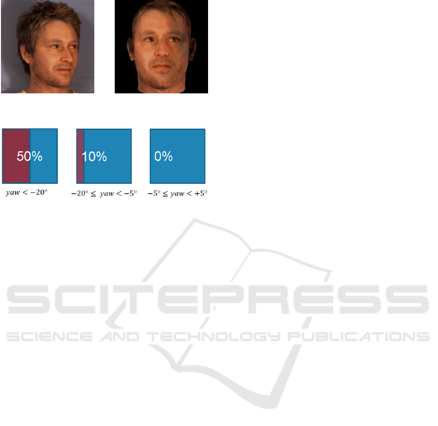
Figure 5: Original (left) and frontalized version (right) of
an image from MUCT.
Figure 6: Masks associated with 3 of the 5 bins of yaw an-
gle. The proportions of discarded pixels (hatched areas) are
written in white.
comparison process because they are poorly visible
on the original non-frontal image. These masks are
transformed into uncertainty matrices on the feature
vectors and are provided to our methods exactly as
explained in Section 5.2.2 for random occlusions.
We use the FRGC images to learn the parameters
of our model (µ, W , S
µ
and S
w
) and test our similar-
ity function on two face datasets with large variations
in pose: PUT (9971 images) and MUCT (3755 im-
ages). We compare our method to standard PCA +
Joint Bayesian by looking at the FNR for a FPR of
0.1%. On PUT, our method obtains a FNR of 2.7%
whereas the baseline achieves 3.1%. On MUCT, the
FNR are respectively 3.4% and 3.6%. First, we re-
mark that error rates on databases with pose variations
are not much higher than those we report on FRGC in
the previous section. This is due to the frontalization
scheme used in this section, FNR are much higher if
comparisons are performed on the original images.
Second, we observe that using an uncertainty-aware
similarity function leads to a notable improvement in
performance on both databases despite the simple and
coarse correspondence between yaw angles and pixel
masks we use.
6 CONCLUSION
In this paper, we have introduced a novel similarity
learning method which, unlike previous approaches,
can take advantage of uncertainty information made
available by the feature extraction process. The two
stages of our method are based on probabilistic mod-
els and we provided EM algorithms to estimate their
parameters.
Our experimental results show the benefit of ex-
plicitly accounting for uncertainty information in sim-
ilarity function learning. We demonstrate the effec-
tiveness of our method on various challenging tasks
such as dealing with images of various resolutions,
pose variations or occlusion.
The main limitation of our work is that our method
requires to be provided uncertainty information about
the data. An interesting direction for future research
is to automatize this task. This could be achieved by
designing a method to make the link between some
image quality measures (for example, local signal-to-
noise ratio at the pixel level) and the data uncertainty
matrices on extracted features.
REFERENCES
Belhumeur, P. N., ao P. Hespanha, J., and Kriegman, D. J.
(1997). Eigenfaces vs. fisherfaces: Recognition us-
ing class specific linear projection. IEEE Transactions
on Pattern Analysis and Machine Intelligence, pages
711–720.
Bi, J. and Zhang, T. (2004). Support vector classification
with input data uncertainty. In NIPS, pages 1651–
1659.
Blanz, V., Grother, P., Phillips, J. P., and Vetter, T. (2005).
Face recognition based on frontal views generated
from non-frontal images. In CVPR, pages 454–461.
Bohn
´
e, J., Ying, Y., Gentric, S., and Pontil, M. (2014).
Large margin local metric learning. In ECCV.
Cao, X., Wipf, D., Wen, F., and Duan, G. (2013). A practi-
cal transfer learning algorithm for face verification. In
ICCV.
Chen, D., Cao, X., Wang, L., Wen, G., and Sun, J. (2012).
Bayesian face revisited: a joint formulation. In ECCV.
Cormode, G. and McGregor, A. (2008). Approximation al-
gorithms for clustering uncertain data. In PODS.
Davis, J. V., Kulis, B., Jain, P., Sra, S., and Dhillon, I. S.
(2007). Information-theoretic metric learning. In
ICML, pages 209–216.
Guillaumin, M., Verbeek, J., and Schmid, C. (2009). Is that
you? metric learning approaches for face identifica-
tion. In ICCV, pages 498–505.
Huang, G. B., Ramesh, M., Berg, T., and Learned-Miller,
E. (2007). Labeled faces in the wild: A database for
studying face recognition in unconstrained environ-
ments. Technical Report 07-49, University of Mas-
sachusetts, Amherst.
K
¨
ostinger, M., Hirzer, M., Wohlhart, P., Roth, P. M., and
Bischof, H. (2012). Large scale metric learning from
equivalence constraints. In CVPR, pages 2288–2295.
Kriegel, H.-P. and Pfeifle, M. (2005). Hierarchical density-
based clustering of uncertain data. In ICDM.
Similarity Function Learning with Data Uncertainty
139

Li, S. Z. and Jain, A. K. (2011). Handbook of Face Recog-
nition 2nd ed. Springer.
Prince, S. J. and Elder, J. H. (2007). Probabilistic linear
discriminant analysis for inferences about identity. In
ICCV.
Ren, J., Lee, S. D., Chen, X., Kao, B., Cheng, R., and Che-
ung, D. W.-L. (2009). Naive bayes classification of
uncertain data. In ICDM.
Shivaswamy, P. K., Bhattacharyya, C., and Smola, A. J.
(2006). Second order cone programming approaches
for handling missing and uncertain data. Journal of
Machine Learning Research, 7:1283–1314.
Sun, Y., Chen, Y., Wang, X., and Tang, X. (2014a). Deep
learning face representation by joint identification-
verification. In NIPS.
Sun, Y., Wang, X., and Tang, X. (2014b). Deep learning
face representation from predicting 10,000 classes. In
CVPR.
Tipping, M. E. and Bishop, C. M. (1999). Probabilistic prin-
cipal component analysis. Journal of the Royal Statis-
tical Society, Series B, 61:611–622.
Tsang, S., Kao, B., Yip, K. Y., Ho, W.-S., and Lee, S. D.
(2011). Decision trees for uncertain data. IEEE Trans-
actions on Knowledge and Data Engineering, 23:64–
78.
Weinberger, K. and Saul, L. (2009). Distance metric learn-
ing for large margin nearest neighbor classification.
Journal of Machine Learning Research, 10:207–244.
ICPRAM 2016 - International Conference on Pattern Recognition Applications and Methods
140