Benchmark Datasets for Fault Detection and Classification in Sensor
Data
Bas de Bruijn
1
, Tuan Anh Nguyen
1
, Doina Bucur
1
and Kenji Tei
2
1
University of Groningen, Groningen, The Netherlands
2
National Institute of Informatics, Tokyo, Japan
Keywords:
Benchmark Dataset, Fault Tolerance, Data Quality, Sensor Data, Sensor Data Labelling.
Abstract:
Data measured and collected from embedded sensors often contains faults, i.e., data points which are not an
accurate representation of the physical phenomenon monitored by the sensor. These data faults may be caused
by deployment conditions outside the operational bounds for the node, and short- or long-term hardware,
software, or communication problems. On the other hand, the applications will expect accurate sensor data,
and recent literature proposes algorithmic solutions for the fault detection and classification in sensor data.
In order to evaluate the performance of such solutions, however, the field lacks a set of benchmark sensor
datasets. A benchmark dataset ideally satisfies the following criteria: (a) it is based on real-world raw sensor
data from various types of sensor deployments; (b) it contains (natural or artificially injected) faulty data
points reflecting various problems in the deployment, including missing data points; and (c) all data points are
annotated with the ground truth, i.e., whether or not the data point is accurate, and, if faulty, the type of fault.
We prepare and publish three such benchmark datasets, together with the algorithmic methods used to create
them: a dataset of 280 temperature and light subsets of data from 10 indoor Intel Lab sensors, a dataset of
140 subsets of outdoor temperature data from SensorScope sensors, and a dataset of 224 subsets of outdoor
temperature data from 16 Smart Santander sensors. The three benchmark datasets total 5.783.504 data points,
containing injected data faults of the following types known from the literature: random, malfunction, bias,
drift, polynomial drift, and combinations. We present algorithmic procedures and a software tool for preparing
further such benchmark datasets.
1 INTRODUCTION
Wireless sensor networks (WSNs) are collections of
spatially scattered sensor nodes deployed in an en-
vironment in order to measure physical phenomena.
The data measured and collected by WSNs is often
inaccurate: external factors will often interfere with
the sensing device. It is then important to ensure the
accuracy of sensor data before it is used in a decision-
making process (Zhang et al., 2010). Recent litera-
ture contributes methods for the detection and clas-
sification of sensor data faults (Shi et al., 2011; Ren
et al., 2008; Li et al., 2011). One could refer to (Zhang
et al., 2010) for a comprehensive survey on fault de-
tection techniques for WSNs. These fault-detection
techniques are evaluated by using datasets from an
own living lab, e.g., (Warriach et al., 2012; Gaillard
et al., 2009), or, more often, using publicly available
datasets, such as those published by Intel Lab (In-
telLab, 2015), SensorScope (SensorScope, 2015), the
Great Duck Island (Mainwaring et al., 2002), and Life
Under Your Feet (LifeUnderYourFeet, 2015).
While those datasets greatly support the research
community of WSNs in general, to the best of our
knowledge, no publicly available datasets are ex-
cellent, general benchmark datasets, in which all
data points are annotated with the ground truth, i.e.,
whether or not the data point is accurate, and, if
faulty, the type of fault and an accurate, “clean” re-
placement value. Thus, researchers must themselves
annotate their dataset in order to obtain the ground
truth; different methods of annotating create different
ground truths, and annotated datasets are not gener-
ally shared. This leads to inconsistencies, even when
using the same raw dataset, in the evaluation of fault-
detection algorithms: the functional performance of a
fault-detection algorithm, measured in the rate of true
positives and the rate of false positives obtained when
experimenting on an annotated dataset.
To address this issue, in this paper we present
Bruijn, B., Nguyen, T., Bucur, D. and Tei, K.
Benchmark Datasets for Fault Detection and Classification in Sensor Data.
DOI: 10.5220/0005637901850195
In Proceedings of the 5th International Confererence on Sensor Networks (SENSORNETS 2016), pages 185-195
ISBN: 978-989-758-169-4
Copyright
c
 2016 by SCITEPRESS – Science and Technology Publications, Lda. All rights reserved
185

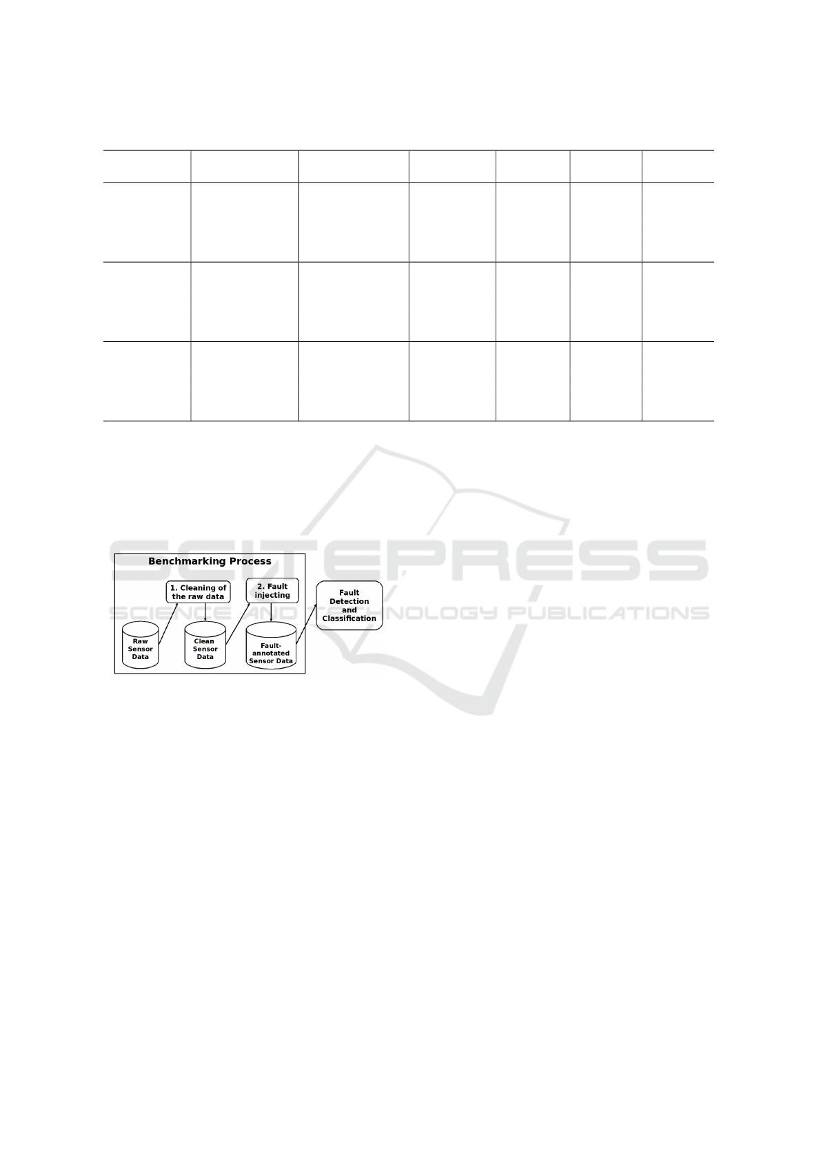
Table 1: Overview of the benchmark datasets.
Missing values Fault types Sensor types Placement
Data Number
samples of sensors
Intel lab
non-interpolated
clean, random,
temperature
indoors 3.980.192 10
and interpolated
malfunction,
and light
bias, drift,
polynomial drift,
mixed
SensorScope
non-interpolated
clean, random,
temperature outdoors 1.063.641 10
and interpolated
malfunction,
bias, drift,
polynomial drift,
mixed
Santander
non-interpolated
clean, random,
temperature outdoors 739.671 16
and interpolated
malfunction,
bias, drift,
polynomial drift,
mixed
a standardised approach to prepare such annotated
benchmark datasets, including 1) cleaning a dataset,
and 2) injecting faults to obtain an annotated dataset
with a selection of faults. Figure 1 gives an overview
of our data benchmarking process, from raw sensor
data to fault-annotated data.
Figure 1: The process of preparing a benchmark dataset.
As the first step, we briefly discuss methods for
cleaning a raw dataset in order to obtain a dataset
without faulty readings; here, no perfect, general
cleaning method exists, and we rely, as also most of
the literature, on visual inspection and some domain
knowledge. After obtaining a clean dataset, we pro-
pose and implement a tool for fault injection based on
the general fault models proposed by (Baljak et al.,
2013). This categorisation is based on the frequency
and continuity of fault occurrences and on observable
and learnable patterns that faults leave on the data.
The models are flexible and applicable to a wide range
of sensor readings. The type of the injected faults is
annotated in the transformed dataset, allowing easier
and meaningful analysis and comparison during algo-
rithm assessment.
The major contributions of this paper are sum-
marised as follows:
• Methods and algorithms to inject faults in clean
datasets on demand based on a generic fault
model.
• Software for the injection of artificial faults in
datasets, supporting users to flexibly create their
own annotated sensor dataset on demand.
• Three large annotated benchmark datasets gener-
ated from the Intel Lab (IntelLab, 2015), Sen-
sorScope (SensorScope, 2015) and the Smart San-
tander (SmartSantander, 2015) deployments, us-
ing our method. The datasets include in total 644
subsets of 5.783.504 annotated readings, injected
with a mix of various fault types.
From the Intel Lab raw data, we extract one week
of temperature and light measurements from each of
10 sensors. The raw data is first cleaned, then we
inject faults. There are 120 fault-injected sets in to-
tal: 10 nodes with each six sets for temperature and
six sets for light. The faults injected are 1) random,
2) malfunction, 3) bias, 4) drift, 5) polynomial drift,
and 6) mixed faults. From SensorScope we use am-
bient temperature data from 10 nodes, resulting in
10 clean datasets and 60 fault-injected datasets us-
ing the same six types of faults as for Intel Lab. The
third benchmark dataset is constructed from a new,
previously unpublished sensor dataset, consisting of
temperature measurements from 16 outdoor sensors
that are part of the Smart Santander project (Smart-
Santander, 2015). This consists of 16 clean datasets
and 96 fault-injected datasets. Furthermore, we offer
the datasets in both interpolated and non-interpolated
form: the non-interpolated dataset uses the original
timestamps and any missing data points are not re-
placed, whereas the interpolated datasets fill in a mea-
SENSORNETS 2016 - 5th International Conference on Sensor Networks
186

surement for each missing value. Table 1 presents an
overview of the benchmark datasets.
The remainder of this paper is structured as fol-
lows: Section 2 explains what types of faults are com-
monly found in wireless sensor data, and how these
faults can be modelled, followed by Section 3 that dis-
cusses the annotation challenges for such dataset and
the proposed approach for benchmarking. Section 4
shows how we obtain a benchmark dataset by apply-
ing our proposed procedure and the software tool. Fi-
nally, we conclude the paper in Section 5.
2 BACKGROUND ON FAULT
MODELS IN SENSOR DATA
As the first step of fault management, it is crucial
to categorise faults. On one hand, by comprehend-
ing the causes, effects, and especially the character-
istics of each fault type onto the data it is possible
to propose suitable fault-tolerance mechanisms to de-
tect, classify, and correct data faults of each type. This
knowledge is also necessary to clean the dataset and
to design functions to inject faults of each type.
2.1 Types of Faults
Fault categorisation techniques vary: several existing
fault taxonomies use different criteria for categorising
a fault. (Ni et al., 2009) give extensive taxonomies
of data faults that include a definition, the cause of
the fault, its duration and its impact onto sensed data.
According to the authors, sensor faults can be clas-
sified into two broad fault types: 1) system faults
and 2) data faults. From a system-centric viewpoint,
faults may be caused by the way the sensor was cal-
ibrated, a low battery level, the clipping of data, or
an environment-out-of-range situation. On the other
hand, data faults are classified as stuck-at, offset, or
gain faults. These same three types of data faults
are denoted short, constant, and noise, respectively,
by (Sharma et al., 2010).
2.2 Fault Models
(Baljak et al., 2013) proposes a complete, general cat-
egorisation based on the the frequency and continu-
ity of fault occurrence and on the observable and
learnable patterns that faults leave on the data. This
categorisation is flexible, and applicable to a wide
range of sensor types. The underlying cause of the
error does not affect this categorisation, which makes
it possible to handle the faults solely based on their
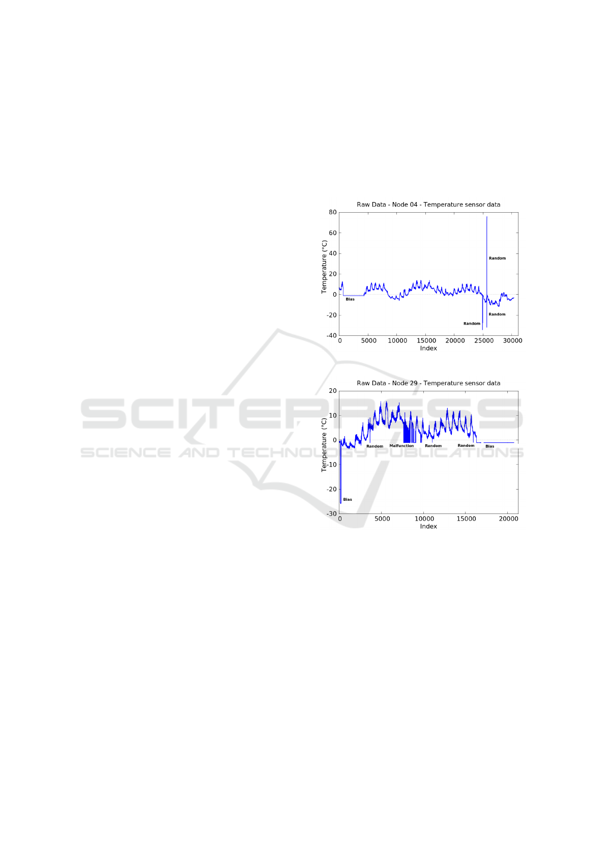
patterns of occurrence on each sensor node. Exam-
ples of several fault types are given in Figure 2. Note
that the figures in this paper display values that are
not necessarily uniformly sampled. While in theory
the sensors report values regularly, reality shows that
quite many values are missing. The gaps that as a re-
sult exist, are usually too small to be visible on the
graphs. Section 4.2 treats this subject in more detail.
(a) One bias and three random faults.
(b) One short duration bias, one long duration bias, one
malfunction and three random faults.
Figure 2: Examples of random, malfunction, and bias faults
taken from the SensorScope dataset, motes 4 (a) and 29 (b).
(Baljak et al., 2013) defines the following models
of data faults:
• Discontinuous – Faults occur from time to time,
and the occurrence of faults is discrete.
– Malfunction – Faulty readings appear fre-
quently. The frequency of the occurrences of
faults is higher than a threshold τ.
– Random – Faults appear randomly. The fre-
quency of the occurrences of faulty readings is
smaller than τ.
• Continuous – During the period under observa-
Benchmark Datasets for Fault Detection and Classification in Sensor Data
187

tion, a sensor returns constantly inaccurate read-
ings, and it is possible to observe a pattern in the
form of a function.
– Bias – The function of the error is a constant.
This can be a positive or a negative offset.
– Drift – The deviation of data follows a learn-
able function, such as a polynomial change.
The fault categorisation in (Baljak et al., 2013),
(Ni et al., 2009) and (Sharma et al., 2010) do overlap.
The fault types can be mapped, as depicted in Table 2,
into one fault or a combination of faults defined using
the other approaches.
An important note about terminology is in order.
Sometimes an outlier is not necessarily a faulty value,
it may be the manifestation of something interesting
happening in the environment. This is not so likely in
case of for example bias faults, but for random faults
this may very well be the case. Distinguishing be-
tween faulty values and interesting events is a diffi-
cult subject. For this paper we will use the term fault,
and leave it to the users of the datasets to use them as
faults, or as anomalies.
Table 2: Relationships between fault models.
(Baljak et (Ni et al., 2009) (Sharma et
al., 2013) Data- System- al., 2010)
centric centric
Random Outlier Short
Random or
Spike
Hardware
Short
Malfunction Low Battery
Bias Stuck-at
Clipping
ConstantHardware
Low Battery
Drift Noise
Low Battery
NoiseHardware
Env. out of range
Bias or
Calibration Noise
Drift
3 ANNOTATION CHALLENGES
AND APPROACH
Two main steps that have to be performed in order to
prepare the dataset for usage are 1) cleaning the raw
data and 2) injecting artificial faults. Cleaning the
data is necessary to ensure that the fault detection al-
gorithms are only executed on known faults, allowing
for consistent evaluations. After that, new faults may
be injected. The proposed fault injection method al-
lows for injecting faults flexibly, as required by the
use case. In the following subsections we explain the
two main steps in more detail.
Table 3: Dataset cleaning techniques in literature.
Visual inspection Run scripts to annotate Domain knowledge No cleaning No mention of cleaning
(Ni et al., 2009)
√
(Hamdan et al., 2012)
√
(Nguyen et al., 2013)
√ √
(Baljak et al., 2013)
√
(Sharma et al., 2010)
√ √
(Warriach et al., 2012)
√
(Ren et al., 2008)
√
(Yao et al., 2010)
√
3.1 Data Cleaning
The main challenge in cleaning the dataset is the fact
that the process can not be fully automated, as no gen-
eral, “perfect” method of detecting sensor data faults
exists. We survey multiple studies in order to obtain
an overview of the data cleaning techniques used in
the field.
3.1.1 Case Studies
Eight studies are surveyed in order to find the most
common techniques used to clean datasets. Table 3
summarises the results. Most studies do not actually
clean the dataset of faults, or they do not formally de-
scribe any cleaning method. Out of the data cleaning
techniques, visual inspection is the most commonly
used: by three out of eight studies. Some mention
running scripts to annotate the data, although no al-
gorithm is described. Some authors employ domain
knowledge on top of visual inspection, which may in-
crease the likelihood that faults are spotted, as domain
experts are more familiar with the underlying phe-
nomenon and thus are more capable in distinguishing
normal data from faults.
3.1.2 Cleaning Guidelines
(Sharma et al., 2010), (Nguyen et al., 2013) and (Yao
et al., 2010) use visual inspection to clean datasets.
A visual presentation of the data can help in locat-
ing faults in large datasets. The human visual per-
ception system is well equipped to spot high-intensity
faults residing in a low-variance phenomenon such
SENSORNETS 2016 - 5th International Conference on Sensor Networks
188

Figure 3: Injected malfunction faults in both temperature and light data, indicated by small arrows. Intel dataset, node 1,
interpolated.
as temperature. However, low-intensity faults resid-
ing in a high-variance phenomenon such as light are
much harder to spot. This visual inspection is best
performed by a domain expert, as he will be better
able to accurately distinguish regular sensor readings
from interesting events and data faults.
Once one or more data faults have been identi-
fied, the data preprocessor needs to decide how to re-
move them. There are two distinct cases. In case the
fault is of short duration, typically less than 10 val-
ues, the faulty values can be easily replaced by inter-
polating between the two correct values at both sides
of the interval. Removing the faults becomes more
complicated when the duration of the faulty interval
is longer, or when the phenomenon is high-variance.
This is due to the fact that more information is ab-
sent as the duration increases, making any estimation
of the original correct value increasingly error prone.
Add to that the fact than some fault-detection methods
(such as those based on time-series analysis) rely on
the fact that the data is measured at equispaced time
intervals, and simply removing the faulty values will
pose problems.
There are several ways the data preprocessor can
remove long-duration faults. It could replace the en-
tire interval with a constant value. This, however, ef-
fectively introduces a bias fault. Alternatively, some
variable offset can be added to this constant value, or
the data preprocessor could replace it with a frame of
readings with somewhat similar values. Of course, it
is safest to not use these intervals at all. There is no
certain way of telling what the faulty values should be
corrected to, and attempting to reconstruct long inter-
vals reduces the integrity of the dataset by introducing
artificial values. In our experience, real world datasets
will start to display more long-duration faults as the
lifetime of the sensor nodes increases. With this in
mind, the best approach is to use sensor data that was
reported before the sensor started to decay.
3.2 Fault Injection
For this paper we choose to use a percentage-based
interval division of the data set. This allows the users
of our proposed tool to precisely specify what parts
of the dataset are to contain certain faults, while still
providing a layer of abstraction over the temporal dis-
tribution of the data. Four vectors, s
r
, s
m
, s
d
, and s
b
,
each contain a number of pairs specifying the start and
end of the intervals of their respective faults: random,
malfunction, drift or bias. These values are percent-
ages. An example vector is: s
r
{(4, 6), (12, 15)}; it
specifies that random faults are to be injected in the
data samples between the first four and six percent
of the dataset, as well as between percentages twelve
and fifteen. This concept is best illustrated by a figure.
Figure 3 displays a dataset where malfunction faults
have been injected into the clean data of node 1 from
the Intel Lab dataset for both temperature and light.
The small arrows indicate where malfunction faults
have been injected, notice that some faults are much
more subtle than others. The faults are only injected
in the user-specified intervals. All four different faults
specified by Baljak’s fault models can be injected in
this fashion, each one having its own parameters to
allow maximum flexibility.
The injection algorithms apply the fundamental
work done by (Sharma et al., 2010). The algorithms
annotate the data with the faults that are injected;
this is an added column to the dataset that stores the
ground truth for each measurement. In the following,
we explain in more detail how the four types of faults
can be injected. Note that the following algorithms
(algorithms 1 to 4) are applied to the data samples in
one of the aforementioned intervals (a pair in s
r
, s
m
,
s
d
or s
b
). In other words, the algorithms are applied to
Benchmark Datasets for Fault Detection and Classification in Sensor Data
189

Table 4: Overview of variables and parameters.
Name Description
s
r
set of intervals for random faults
s
m
set of intervals for malfunction faults
s
d
set of intervals for drift faults
s
b
set of intervals for bias faults
δ
r
density (percentage) of random
faults in the intervals
i
r
intensity vector for random faults
n
m
noise intensity parameter
for malfunction faults
i
d
intensity vector for drift faults
n
d
noise intensity parameter for drift faults
n
b
noise intensity parameter for bias faults
i
b
intensity vector for bias faults
m
b
mean value for bias faults
S subset of the clean data
I
vector containing (value, annotation)
pairs representing an annotated,
fault-injected version of S
a subset of the clean dataset. This subset is denoted by
S. It is not specific to any fault type, it is merely a rep-
resentation of some subset of the clean data. Table 4
summarises the used variables and parameters.
3.2.1 Random Fault
Random faults often occur in an isolated fashion. We
propose a method that allows injecting random faults
with a user-specified density, δ
r
, in the data samples
from an interval in s
r
. These data samples are denoted
by S. The density parameter δ
r
determines the per-
centage of readings within S that are to be a random
fault. Let k be some index for S. A value S
k
in S is
transformed into an annotated random fault I
k
based
on formula 1:
I
k
= (S
k
(1 + intensity), “random”) (1)
where intensity is a value from the vector of intensi-
ties, specified by the user as parameter i
r
. A random
intensity is chosen from i
r
for each fault. This is im-
plemented in Algorithm 1.
3.2.2 Malfunction Fault
Malfunction faults do not rely on a density parame-
ter, as they typically affect all readings within an in-
terval. Malfunction faults are defined as an interval
of measurements that display a higher variance than
normal. To recreate this increased variance, we com-
pute the variance over the original measurements in S:
σ
original
. This is then used to obtain a value from the
normal distribution with mean zero and the computed
Algorithm 1: Injecting Random Faults.
Input: S[1..N]: subset of the clean dataset, a vector
of N measurements
δ
r
: density parameter
i
r
: intensities vector
Output: I[1..N]: vector of (value, annotation) pairs
representing N annotated random-fault-injected
sensor readings
1: for i = 1 to N do
2: p ← random percentage ∈ [0,100]
3: r ← random index ∈ [1,|i
r
|]
4: if p > δ
r
then
5: I[i] ← (S[i], “clean”)
6: else
7: newValue ← S[i] ∗(1 + i
r
[r])
8: I[i] ← (newValue, “random”)
9: end if
10: end for
11: return I
variance, which is then multiplied by a user-specified
intensity, n
m
. This new value is added to the original
value to obtain the injected fault:
I
k
= (S
k
+ N (0, σ
2
original
) ∗n
m
, “malfunction”) (2)
Note that we model malfunction faults by making an
assumption as to the expected probabilistic distribu-
tion of malfunction faults. However, we have no con-
crete knowledge as to which distribution gives the
most accurate model for a particular type of faults and
a particular type of sensor; we chose a normal distri-
bution as the most likely.
This method for the injection of malfunctions is
implemented in Algorithm 2.
Algorithm 2: Injecting Malfunction Faults.
Input: S[1..N]: subset of the clean dataset, a vector
of N measurements
n
m
: noise intensity parameter
Output: I[1..N]: vector of (value, annotation)
pairs representing N annotated malfunction-fault-
injected sensor readings
1: v ← variance of S
2: for i = 1 to N do
3: newValue ←S[i] + N (0, v
2
) ∗n
m
4: I[i] ← (newValue, “malfunction”)
5: end for
6: return I
3.2.3 Drift Fault
Drift faults can be injected in multiple ways. One
way to do it is by using a polynomial to model the
drift fault. The polynomial consists of a number of
SENSORNETS 2016 - 5th International Conference on Sensor Networks
190

coefficients: a
0
, . . . , a
n
, and a number of variables:
x
0
, . . . , x
n
. The summation of their products forms the
polynomial model. Substituting x for k and adding the
original value from S, we obtain the following equa-
tion for the new value:
I
k
= (S
k
+
n
∑
i=0
a
i
k
i
, “poly-drift”) (3)
Another method that deviates from Baljak’s fault
models is by injecting drift faults as a sequence of
values with an offset to the original data, with some
variance added to it. The formula for this method is
as follows:
I
k
= (S
k
+ N (0, σ
2
original
) ∗n
d
+ offset, “drift”) (4)
The offset is obtained by taking the first measurement
from the interval and multiplying it with a random in-
tensity from the user-specified intensities i
d
. n
d
de-
termines the amount of noise that is added to the drift
fault. Formula 4 is implemented in Algorithm 3.
Algorithm 3: Injecting Drift Faults.
Input: S[1..N]: subset of the clean dataset, a vector
of N measurements
i
d
: intensities vector
n
d
: noise intensity parameter
Output: I[1..N]: vector of (value, annotation) pairs
representing N annotated drift-fault-injected sen-
sor readings
1: r ← random index ∈ [1,|i
d
|]
2: v ← variance of S
3: offset ← S[1] ∗i
d
[r]
4: for i = 1 to N do
5: newValue ←S[i] + N (0, v
2
) ∗n
d
+ offset
6: I[i] ← (newValue, “drift”)
7: end for
8: return I
3.2.4 Bias Fault
A bias fault is defined as a number of measurements
that display little to no variance, usually accompanied
by some offset to the expected value. There are two
ways to inject a bias fault, both have the option to add
some variance with intensity n
b
:
1. Supply a value m
b
that is to be used as the new
mean:
I
k
= (m
b
+N (0, σ
2
original
)∗n
b
, “mean-bias”) (5)
2. Supply a factor i
b
that will be multiplied with the
original mean of the measurements in the time
frame:
I
k
= (i
b
∗µ
original
+ N (0, σ
2
original
) ∗n
b
, “bias”)
(6)
Formula 6 for injecting bias faults is implemented in
Algorithm 4.
Algorithm 4: Injecting Bias faults.
Input: S[1..N]: subset of the clean dataset, a vector
of N measurements
n
b
: noise intensity parameter
i
b
: intensities vector
Output: I[1..N]: vector of (value, annotation) pairs
representing N annotated bias-fault-injected sen-
sor readings
1: r ← random index ∈ [1,|i
b
|]
2: v ← variance of S
3: o ← original mean of S
4: newMean ← o * i
b
[r]
5: for i = 1 to N do
6: newValue ←newMean + N (0, v
2
) ∗n
b
7: I[i] ← (newValue, “bias”)
8: end for
9: return I
4 THE DATASET
We implement the fault injection methods in Java. A
publicly available release of the three datasets is avail-
able at http://tuananh.io/datasets.
4.1 Cleaning Raw Data from the
Datasets
We visually inspect the raw data time series to iden-
tify the characteristics of correct readings, as well as
those of random, malfunction, bias, and drift faults.
The approach for cleaning the Intel Lab dataset is
slightly different from the one used for SensorScope.
For the Intel Lab dataset, we determined that the first
week was free of long-duration faults for all nodes,
and thus decided to select the readings from this in-
terval for our benchmark dataset. Figure 4 shows the
selected first week of clean data from node 1 of the In-
tel Lab dataset. Note that the gaps are clearly visible,
these are points where values are missing. The short-
duration faults are manually removed by interpolating
between the correct neighbouring values. The Sen-
sorScope dataset contained some nodes that displayed
long-duration faults within the first week of deploy-
ment. In this case we decided to select the read-
ings from a custom interval for each node, up until
the first long duration interval is present. The conse-
quence is that some of the cleaned nodes contain more
readings than others. Again we removed the short-
duration fault by hand, by interpolating between the
Benchmark Datasets for Fault Detection and Classification in Sensor Data
191

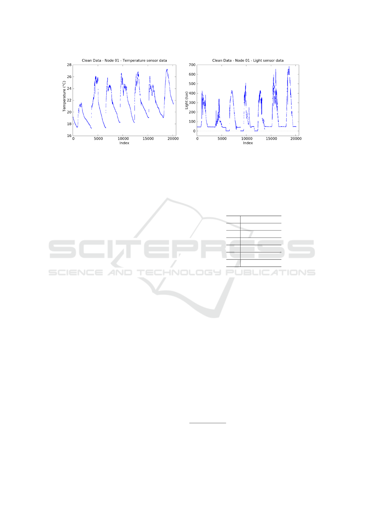
Figure 4: Clean temperature data (left) and light data (right) from mote 1 of the Intel Lab dataset.
neighbouring values. For the Smart Santander dataset
we selected a period of data of about two weeks that
was free of faults. In all three cases we have relied
mainly on a smart selection of data subsequences, so
as to minimize the amount of faults that have to be
removed.
4.2 Uniform Data Frequency
Some fault detection methods, such as seasonal
Auto-Regressive Integrated Moving Average
(ARIMA) (Nguyen et al., 2013; Box et al., 2013),
call for a fixed number of data samples in a certain
period, or season. The three datasets in their original
form contain many missing values, which interferes
with these methods. Because sensor technologies
continue to improve, we expect that missing values
will become rarer in the future.
It is for these reasons that we provide the bench-
mark datasets in two forms: the first form uses
the timestamps and measurements from the original
dataset, and thus has missing data points. The sec-
ond form ensures that a measurement is present for
each expected timestamp. For example, if the sensor
is supposed to report a measurement every five min-
utes, the datasets of the second form will contain a
measurement for every five minutes within the inter-
val. If a timestamp is missing, a new data sample will
be created with the measurement interpolated in a lin-
ear fashion.
4.3 Annotated Fault-Injected Datasets
The implementation details of the four algorithms are
presented in Algorithms 1 to 4. The parameters used
for the algorithms are listed in the algorithm listings.
These parameters are obtained through trial and error;
we adjusted them until they resulted in the best repre-
sentation of real world faults for these types of sensed
data. Note that these parameters work for these par-
ticular datasets, they may not necessarily work for all
datasets. So while the method for injecting faults is
general, the parameters will often be specific to the
datasets.
Table 5: Algorithm parameters.
δ
r
0.2
i
r
(1.5, 2.5)
n
m
1.5
i
d
(−2, −1, 1, 2)
n
d
2.0
n
b
0
i
b
(1.5)
In the provided benchmark datasets, the percent-
age of faulty readings differs per fault type. In case
of injected drift faults, 20% of the readings are faulty.
In case of injected random faults 20% of the dataset
is affected by random faults. The intervals that are af-
fected by random faults in turn have a density of 20%
faults, resulting in 4% of actual random faults. Bias
and malfunction faults are both injected in 21% of the
readings, while the mixed datasets consist of 4% ran-
dom faults
1
, 4% drift faults, 6% malfunction and 6%
bias faults. Figure 5 graphically illustrates datasets
with faults injected of types random, drift, polynomial
drift, bias and mixed fault types. These are injected
over the temperature and light sensor data of node 1
from the Intel dataset (shown in Figure 4).
1
Note that again, this means that 4% is affected by a
random fault and 20% of this 4% is an actual random fault,
resulting in 0.8% actual random faults.
SENSORNETS 2016 - 5th International Conference on Sensor Networks
192

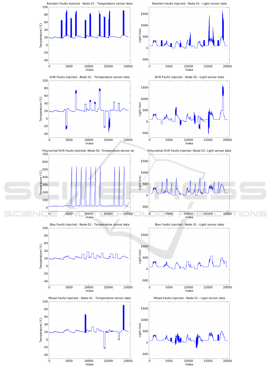
Figure 5: Five different fault types injected in node 1 of the Intel Lab dataset (left: temperature sensor data; right: light
sensor data). Interpolated data.
Benchmark Datasets for Fault Detection and Classification in Sensor Data
193

5 CONCLUSIONS, DISCUSSION,
AND FUTURE WORK
Summary of Contribution and Critical Discus-
sion. The literature does not currently give a struc-
tured methodology for cleaning a raw dataset of sen-
sor readings, and especially obtaining an annotated
dataset of readings which includes data faults in con-
figurable patterns. Without this methodology, studies
which design and evaluate algorithms for anomaly de-
tection, classification, and correction in sensor data is
difficult to evaluate comparatively.
Cleaning a given dataset is ideally done via the
resource-heavy process comparing the sensor data
against data acquired concurrently by a second, cal-
ibrated, high-fidelity sensor, which is able to col-
lect digital data, and either download it over a net-
work, or store large datasets in memory. However,
an ideal such second sensor is rarely available in
real-world deployments, and arguable all the sensor
datasets currently available for experimentation have
been cleaned via an unstructured process which com-
bines a degree of domain knowledge with a form of
basic inspection of the data. This process is error-
prone, and may not differentiate (for all types of phys-
ical phenomena sensed) between legitimate faults in
the data and true anomalous conditions in the envi-
ronment. Other means for classifying raw data points
are surveyed in (Zhang, 2010).
This paper does not contribute a data-cleaning
methodology, but provides a framework to prepare
annotated datasets with configured injected faults,
which are well suited for then evaluating fault-
detection methods. The framework requires a clean
dataset in the input. The datasets we publish here have
used as clean data some subsets of raw datasets which
we have judged, using our own domain knowledge
and visual inspection, to have been the least affected
by faults in the sensing system, and which thus re-
quired minimal manual cleaning and interpolation for
missing values.
We provide three benchmark datasets for the eval-
uation of fault detection and classification in wire-
less sensor networks, and a Java library which im-
plements configurable fault-injection algorithms. The
first benchmark dataset includes 280 subsets of tem-
perature and light sensors of 10 nodes extracted from
the Intel Lab raw data. The second benchmark dataset
includes 140 subsets of ambient temperature sensors
extracted from the SensorScope dataset. The third
benchmark dataset includes 224 subsets of tempera-
ture measurements obtained from 16 sensors as part
of the Smart Santander project. The three bench-
mark datasets total 5.783.504 data samples, covering
six types of faults that have been observed in sen-
sor data by prior literature. Faults are injected using
known, generic fault models. We publish the datasets
at http://tuananh.io/datasets. We believe that all pa-
pers listed in table 3 would have benefited from using
such annotated datasets.
This paper attempts an initial, systematic treat-
ment of the problem of the missing annotated
datasets. Its main limitation lies in the fact that the an-
notated datasets have been obtained based on cleaned
sensor data that is still not entirely guaranteed to be
free of all faulty readings.
Future Work. We plan to extend the current
datasets two-fold: (a) by processing and publish-
ing sensor datasets pertaining to physical phenomena
other than light and temperature, and (b) by prepar-
ing annotated datasets based on cleaned datasets with
a better guarantee of correctness. Also, we aim at de-
veloping a software tool of a user-friendlier nature,
for configuring the fault injection algorithms.
ACKNOWLEDGEMENT
The work is supported by 1) the FP7-ICT-2013-EU-
Japan, Collaborative project ClouT, EU FP7 Grant
number 608641; NICT management number 167
and 2) the Dutch National Research Council En-
ergy Smart Offices project, contract no. 647.000.004
and 3) the Dutch National Research Council Beijing
Groningen Smart Energy Cities project, contract no.
467-14-037.
REFERENCES
Baljak, V., Tei, K., and Honiden, S. (2013). Fault classi-
fication and model learning from sensory readings –
framework for fault tolerance in wireless sensor net-
works. In Intelligent Sensors, Sensor Networks and
Information Processing, 2013 IEEE Eighth Interna-
tional Conference on, pages 408–413.
Box, G. E., Jenkins, G. M., and Reinsel, G. C. (2013). Time
Series Analysis: Forecasting and Control. Wiley.com.
Gaillard, F., Autret, E., Thierry, V., Galaup, P., Coatanoan,
C., and Loubrieu, T. (2009). Quality control of large
argo datasets. Journal of Atmospheric and Oceanic
Technology, 26.
Hamdan, D., Aktouf, O., Parissis, I., El Hassan, B., and Hi-
jazi, A. (2012). Online data fault detection for wireless
sensor networks - case study. In Wireless Communi-
cations in Unusual and Confined Areas (ICWCUCA),
2012 International Conference on, pages 1–6.
SENSORNETS 2016 - 5th International Conference on Sensor Networks
194

IntelLab (2015). The Intel Lab at Berkeley dataset.
http://db.csail.mit.edu/labdata/labdata.html.
Li, R., Liu, K., He, Y., and Zhao, J. (2011). Does fea-
ture matter: Anomaly detection in sensor networks.
In Proceedings of the 6th International Conference
on Body Area Networks, BodyNets ’11, pages 85–91,
ICST, Brussels, Belgium, Belgium. ICST (Institute for
Computer Sciences, Social-Informatics and Telecom-
munications Engineering).
LifeUnderYourFeet (2015). The Life Under Your Feet
dataset. http://www.lifeunderyourfeet.org/.
Mainwaring, A., Culler, D., Polastre, J., Szewczyk, R.,
and Anderson, J. (2002). Wireless sensor networks
for habitat monitoring. In Proceedings of the 1st
ACM International Workshop on Wireless Sensor Net-
works and Applications, WSNA ’02, pages 88–97,
New York, NY, USA. ACM.
Nguyen, T. A., Bucur, D., Aiello, M., and Tei, K. (2013).
Applying time series analysis and neighbourhood vot-
ing in a decentralised approach for fault detection and
classification in WSNs. In SoICT’13, pages 234–241.
Ni, K., Ramanathan, N., Chehade, M. N. H., Balzano, L.,
Nair, S., Zahedi, S., Kohler, E., Pottie, G., Hansen,
M., and Srivastava, M. (2009). Sensor network data
fault types. ACM Trans. Sen. Netw., 5(3):25:1–25:29.
Ren, W., Xu, L., and Deng, Z. (2008). Fault diagnosis
model of WSN based on rough set and neural network
ensemble. In Intelligent Information Technology Ap-
plication, 2008. IITA ’08. Second International Sym-
posium on, volume 3, pages 540–543.
SensorScope (2015). The SensorScope dataset.
http://sensorscope.epfl.ch/.
Sharma, A. B., Golubchik, L., and Govindan, R. (2010).
Sensor faults: Detection methods and prevalence in
real-world datasets. ACM Transactions on Sensor Net-
works (TOSN), 6(3):23.
Shi, L., Liao, Q., He, Y., Li, R., Striegel, A., and Su, Z.
(2011). Save: Sensor anomaly visualization engine.
In Visual Analytics Science and Technology (VAST),
2011 IEEE Conference on, pages 201–210.
SmartSantander (2015). Smart Santander.
http://www.smartsantander.eu/.
Warriach, E., Aiello, M., and Tei, K. (2012). A ma-
chine learning approach for identifying and classify-
ing faults in wireless sensor network. In Compu-
tational Science and Engineering (CSE), 2012 IEEE
15th International Conference on, pages 618–625.
Yao, Y., Sharma, A., Golubchik, L., and Govindan, R.
(2010). Online anomaly detection for sensor systems:
A simple and efficient approach. Performance Evalu-
ation, 67(11):1059–1075.
Zhang, Y. (2010). Observing the Unobservable - Dis-
tributed Online Outlier Detection in Wireless Sensor
Networks. PhD thesis, University of Twente.
Zhang, Y., Meratnia, N., and Havinga, P. (2010). Out-
lier detection techniques for wireless sensor networks:
A survey. Communications Surveys Tutorials, IEEE,
12(2):159–170.
Benchmark Datasets for Fault Detection and Classification in Sensor Data
195