
Bayesian Inventory Planning with Imperfect Demand Estimation
in Online Flash Sale
Ted Tao Yuan
1
, Michelle Cai
2
and Daniel Kao
2
1
Vipshop US, 2550 North First Street, Suite 300, San Jose, CA 94131, U.S.A.
2
Guangzhou VIP Information Technology Co., Ltd, 20 Huahai Road, Liwan District, Guangzhou, China
Keywords: Newsvendor Model, Flash Sale, eCommerce, Machine Learning, Bayesian Inference, Stochastic Model
Applications in Inventory Management and Automation.
Abstract: Daily deal, or flash sale, websites offer limited quantity of selected brands and products for a short period of
time. The idea is that short-term sales event of branded products drives consumer interest. Flash sale sites like
vip.com negotiate great deals from various vendors on a limited quantity of selected products. In operation,
all merchandises need to be allocated to regional warehouses before a short-term sales event starts. The variety
and quantity of merchandises change significantly from one sales event to another. Unsold items are typically
shipped back to vendors after the sales event ends. In this paper, we discuss the design and implementation
of a regional warehouse merchandise allocation model and strategy to maximize sales conversion rate. Our
work reveals the uniqueness of inventory planning of flash sale and its similarity to that of general online
retailers. Our machine learning prediction models and Bayesian Updating strategy are highly valuable to the
improvement of regional warehouse efficiency and customer experience in dealing with highly volatile flash
sale inventory.
1 INTRODUCTION
Online ecommerce retailers usually make their
product offerings available with plenty of inventory
for customers. In the business model, supply quantity
and price of a product can be adjusted according to
demand from buyers over time, such that it operates
according to the law of demand. In many cases,
demand curve
(O'Sullivan and Sheffrin, 2005) can be
constructed from user behavioural and transaction
data available at different price points. The variety
and quantity of products of online retailers are
typically maintained at certain levels from time to
time based on demand and price predictions.
Flash sale, also known as deal-of-the-day, is a
recently popular ecommerce model with time- and
quantity-limited offerings of discounted
merchandises. The flash sale business model is built
on short-term shallow inventory with limited quantity
of branded products at highly discounted prices. The
limited availability and ever-changing conglomerate
of selected merchandises daily on display at a flash
sale site, which is partitioned by geographic regions
in the discussion, makes it difficult to accurately
predict demand needed for the site’s day-to-day
operation from merchandise selection to online
display ranking and inventory planning. For example,
before a scheduled sales event starts, what
merchandises from vendors to be included in the
event? How to pre-distribute tens of thousands of
selected SKUs (stock keeping unit, a distinct item for
sale), each with small or fixed available quantity, to
N regional warehouses, such that it reduces operation
cost, maximizes overall sales conversion rate (max
profit for the business) and at same time achieves best
user experience by shipping from a warehouse closest
to a buyer?
In this paper, we present a study on flash sale
regional inventory planning based on machine
learning (ML) statistical demand estimation, as well
as an enhancement strategy using Bayesian Updating
(
DeGroot and Schervish, 2002) that can take the ML
estimate with a prior. The Bayesian Updating
estimate may have bigger impact to the merchandise
allocation among regional warehouses than the ML
model estimates on flash sale’s constantly changing
inventory. Discussion of flash sale inventory
challenges in business operations can be found in a
recent article (Savino, 2011).
Yuan, T., Cai, M. and Kao, D.
Bayesian Inventory Planning with Imperfect Demand Estimation in Online Flash Sale.
DOI: 10.5220/0005632303430348
In Proceedings of 5th the International Conference on Operations Research and Enterprise Systems (ICORES 2016), pages 343-348
ISBN: 978-989-758-171-7
Copyright
c
2016 by SCITEPRESS – Science and Technology Publications, Lda. All rights reserved
343

2 DEMAND ESTIMATION
One of the ecommerce business key performance
indices is to maximize sales conversion rate of
merchandise on site. The conversion rate can be
measured by the quantity sold divided by total
quantity available for a SKU during a sales event. It
can be affected by many business processes, from
product selection to its ranked display on site, and to
the timely delivery to customers. All else being equal,
how can we improve overall sales conversion rate by
improving regional merchandise distribution
planning? Specifically, given some quantity of a SKU
that we may have limited past sales knowledge, we
need to determine the quantity allocation ratio for pre-
distribution of the merchandise to each regional
warehouse.
Although flash sale is unique in its business
operation, merchandise sell-or-not is inherently
determined by the quality of a product and demand
and display ranking factors such as brand recognition,
fashion, price discount, seasonality, color, size
preference by region, etc. To determine regional
quantity allocation ratio based on the demand
estimation of sales of merchandise, we built ML
models to predict the regional demand for a SKU.
There has been a large literature on multi-echelon
distribution systems and inventory allocation (
Ghiani
et al., 2004). In our distribution configuration, we
assume overall supply is given and must be pre-
distributed to customer-facing regional warehouses
(fulfilment centers) before a flash sale event starts.
Due to the short period of a flash sale and business
policy, transferring merchandises between regional
distribution warehouses, or warehouse serving
customers in a different region, is typically not
allowed.
2.1 Newsvendor Model
Newsvendor, or newsboy or single-period
(Stevenson, 2009) or perishable (Malakooti, 2013),
model can be traced back to a paper (Edgeworth,
1888) where Edgeworth used central limit theorem to
estimate the optimal cash reserves to satisfy random
withdrawals from depositors.
In the Newsvendor model (Arrow et al., 1951) of
inventory optimization, it concerns how many copies
of the day's paper to stock in the face of uncertain
demand and knowing that unsold copies will be
worthless at the end of the day. The optimal solution
is to statistically balance the cost of being
understocked (a loss of sale) with inventory cost of
being overstocked. By and large, this simple model is
applicable to retail inventory management (Gallego et
al., 1993). We can develop business specific supply
and demand estimation to plug into the model.
Figure 1 shows that the uncertainty around the
minimum cost in the Newsvendor model is greatly
affected by the variance of the underlying demand
and supply estimation. The decreasing linear dotted
line at left represents the cost of sales loss due to
understock when demand is greater than supply, the
increasing linear dotted line at right represents
inventory cost due to overstock when demand is less
than supply. When demand equals supply, there is no
sales loss or leftovers and the cost is zero. These are
the cases when the demand and supply are estimated
accurately without uncertainty. The three curves
show the minimum costs under uncertainty due to the
fluctuation of demand and supply. The lowest curve
is when the demand and supply fluctuation variance
is low, and the top curve is when variance is high. We
see as demand and supply variance gets higher, both
the expected minimum cost and the “safety” stock
level increase, and the cost function becomes much
more flat. In other words, the impact of the optimal
solution to business diminishes fast if the demand and
supply estimation has large statistical variance.
Figure 1: Cost under uncertain demand (D) and supply (S).
In flash sale, it usually acquires fixed quantity of each
SKU for a short-term sales event. It boils down to
stochastic demand estimation at each regional
warehouse based on historical sales and viewing
records if exist, and from aggregated statistics of sales
of similar merchandise or product category,
seasonality, regional discriminative factors such as
size, color, fashion, etc.
Among many choices, we choose to train non-
linear, non-parameterized machine learning models
using gradient boosted decision trees (GBDT)
(Friedman, 1999) to predict demand and regional
warehouse merchandise allocation ratio based on past
sales and sales proportion ratio in the regions. Our
training datasets are typically in the size of millions
with features extracted from brand, product and
ICORES 2016 - 5th International Conference on Operations Research and Enterprise Systems
344
recent sale transaction databases in the Chinese
market. We discuss two ML models that are tightly
correlated with slightly different business and
operation interests.
2.2 ML Model to Predict Regional
Warehouse Allocation Ratio of a
SKU
In the model, we try to infer a SKU’s sales proportion
ratio at a regional warehouse from historical sales
data. The sales proportion ratio is the sold quantity at
a regional warehouse divided by the total sales across
all regions. The machine-learning model
(GBDT_ALR) is summarized in the following
relation,
sales proportion ratio: y = function(
region, brand, product sales history, product
attributes, clicks and views, …)
with function f estimated by regression to minimize a
loss function ψy,fx,
argmin
,
,
We plan to use the inferred sales proportion ratio
as the guidance to merchandise allocation among
different regions.
We used GBM package in R to train the GBDT
model. The training set consists of millions of
randomly selected samples from the past sales
records, and the target is computed from the past sales
proportion ratio at regional distribution centers. It is
noted that we favor samples with larger sales quantity
and repeated sales that have less variance, and
samples with overall uniform sales conversion rates
across warehouses for SKUs. We gave them higher
sample weights in GBDT model training. We
adjusted the learn rate (shrinkage factor) and number
of decision trees to generate the best training result.
In offline test validation, the model gives us
overall 80% accuracy when we compare predicted
sold quantity with actual sales in our test data set. It
reveals for flash sale, in clothing, shoes and
accessories for example, the most important factors
are brand recognition, size differential by region (i.e.,
northern prefers larger sizes, southern prefers
smaller), and product category overall sales rate etc.
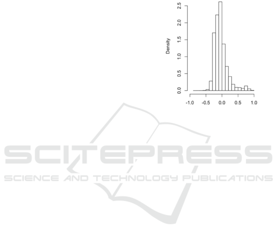
Figure 2 is a density plot of the difference (x-axis)
between the predicted sales proportion ratio and
actual SKU allocation ratio. The SKU allocation ratio
is simply the percentage of the merchandise that we
pre-distributed to the region. The distribution is
generally in a Gaussian form, which tells us our
distribution allocation ratio did generally agree with
sales proportion ratio. It has room to improve as it
slightly weighted to the left (overstocked), had small
tail on the right (understocked), also a sizeable sigma
(~0.25).
Figure 2: Prediction vs actual allocation ratio.
When applied to production, we more focused on
sales loss due to the misplacement of goods, i.e.,
overstock one region, understock others. To minimize
sales loss, business usually sets portion of the total
supply of a SKU under the ML pre-distribution tests.
For that matter, we have two measures for each test,
a “call-back” rate which is defined as the percentage
of the pre-distributed goods that did not sell and had
to be shipped back and returned to vendors, and a
sales coverage rate which is defined as the percentage
of the pre-distributed and sold goods among all sold
goods for a brand. In our environment, logistics sets
priority and requires the call-back rate to be less than
10%. After the call-back rate meets the requirement,
we can gradually increase the pre-distributed portion
to increase the sales coverage rate. In our tests, the
sales coverage rate can be anywhere from 15% to
100% for various brands.
2.3 ML Model to Predict Sales
Conversion Rate of a SKU
As conversion rate is the main business interest, we
also built a GBDT model to predict sales conversion
rate (GBDT_SCR). The goal is to learn the following
relationship,
sales conversion rate: y = function(
region, brand, product sales history, product
attributes, clicks and views, …)
where function f is estimated using the R/GBM
package.
Bayesian Inventory Planning with Imperfect Demand Estimation in Online Flash Sale
345

The regional sales conversion rate of a SKU
equals to the sold quantity divided by quantity
available to sell in the regional warehouse. The model
prediction can also be used to guide SKU’s allocation
so that more items are pre-stocked to a regional
warehouse with higher predicted sale probability.
Usage of the conversion rate prediction model in
merchandise allocation will be discussed in section 3.
The training data set can be assembled in pretty
much the same way as the GBDT_ALR model with
similar features except the target values. We have
tuned the training parameters such as learn rate,
number of trees as well as distributions (Gaussian for
regression and Bernoulli for classification) in the
GBDT algorithm to achieve best training result. The
classifier model has an AUC value 0.84 with the test
data set. As the model is equivalent to learning an
item’s probability of sale in a region, it reveals a
different set of important factors from the sales
proportion ratio model.
2.4 Comparison of the GBDT Models
Table 1 lists the variables of each model in each
column sorted by importance,
Table 1: Top important factors.
Sales Allocation Model
(GBDT_ALR)
Sales Conversion Model
(GBDT_SCR)
Warehouse region ID Brand name
Brand name Last time sale quantity
Brand regional past sales
proportion
Last three month SKU
sale quantity
Total stock quantity Last three month product
sale quantity
Similar size item regional
sales proportion
Total stock quantity
… …
3 BAYESIAN UPDATING
The ML model GBDT_ALR discussed above gives
us a fairly good estimation to determine item pre-
distribution allocation ratio based on sales proportion
ratio for goods with larger quantity of items and
repeated sales. However, major portion of our daily
flash sale merchandise SKUs are either newly arrivals
and/or with small total available quantity (typically <
10) from various vendors. If evenly distributed to
warehouses, it is normal that there can be only 1 or 2
items per SKU available for each regional warehouse.
In such cases, the training dataset samples have much
larger variance on the target labels and certain sales
features, and the model was not optimally trained
with lower statistical confidence on the major portion
of the inventory.
In some way, it can be related to the well-known
Bullwhip/Forrester effect (Hau et al., 1997) that exists
in supply chain management systems. Seasonality,
product life cycle and pure demand uncertainty all
contribute.
With the imperfect demand estimation and other
business specific requirements, we sometimes take
subjective human intervention by injecting rules to
enhance the prediction results. We are also
continuously exploring new factors that can further
improve the precision of the models.
The main issue here is the lack of, or short demand
history for many SKUs. Statistically, it is not proper
to assume one-time sold-out of 1 or 2 items at one
warehouse implies 100% sales conversion rate during
next sales time or at higher inventory levels. The
randomness of sales seems impacting more on the
GBDT_ALR sales proportion model. This leads us to
consider other ways to enhance the ML prediction
models, specifically the Bayesian Updating (Gelman
et al., 2003) approach.
3.1 Bayesian Updating
We believe demand estimation D can be measured by
observed sales quantity. Assuming we have N=3
regional merchandise distribution warehouses, the
total demand estimation D of a SKU is the sum of the
demand estimation in each region D(i),
D = D
1
+ D
2
+ D
3
= S(1) *
p
(1) + S(2) *
p
(2)+S(3)*
p
(3)
(1)
where S(i) is the item’s allocated quantity in region i,
p(i) is the item’s sales conversion rate in the region.
The total quantity of a SKU available for sell is S
= S(1) + S(2) + S(3). The overall sales conversion rate
of the SKU across all regions is
p=
D
S
=
S
1
S
*p
1
+
S
2
S
*p
2
+
S
3
S
*p
3
=r
1
*p
1
+r
2
*p
2
+r
3
*p
3
= r
i
*p(i)
N
i=1
where r(i) = S(i)/S is the SKU’s allocation ratio in
region i, and
∑
r
i
=1
N
i=1
. r(i) is used in the pre-
distribution planning to determine the stock quantity
at the regional warehouse. The overall sales
conversion rate of a flash sale is the weighted average
of all its SKUs’ sales conversion rates.
We can interpret r(i) as the probability of a SKU
ICORES 2016 - 5th International Conference on Operations Research and Enterprise Systems
346
item being distributed to region i. and p(i) as the
probability that it will be sold in the region. From
Bayes’ theorem
(Gelman et al., 2003), the probability
of a SKU being allocated to region i knowing its
probability of being sold in the region is
|
|
∗
∑
∗
(2)
This provides us the formula to compute future
warehouse allocation ratio for the SKU with updated
knowledge of sales conversion rate and prior
warehouse inventory level. The updated conversion
rate knowledge can be acquired either through online
monitoring and measurement of the actual sales, or
from the GBDT_SCR conversion rate model
described in section 2.3 based on past online sales
data.
3.2 Inventory Planning and Online
Monitoring
As Bayesian, we could start with equal distribution
among warehouses. We can have better estimation
given the ML sales conversion model. To illustrate,
lets say our initial sales conversion rate estimates
from the GBDT_SCR model output are
1
0,
2
80%
3
30%
If we assume equal prior, from Bayes’ theorem,
1
0%,
2
73%
3
27%
With minor rounding and human judgment in reality,
we would choose a SKU’s warehouse allocation ratio
for the 3 regions as
1
5%,
2
70%
3
25%
We would have a forecast estimate of the SKU’s
overall sales conversion rate as p =
∑
r
i
*pi =
63.5% with this allocation.
After the sales event starts, lets say we measure
the actual sales conversion rate at the end of day 1 in
each region of the SKU as
1
0%,
2
90%
3
20%
We can update the SKU’s sales conversion estimate
as p' =
∑
r
i
*p'i = 68%. We can continuously
update and monitor the SKU’s overall conversion rate
p", p''', … with new regional sales measurements at
the end of day 2, 3, and so on.
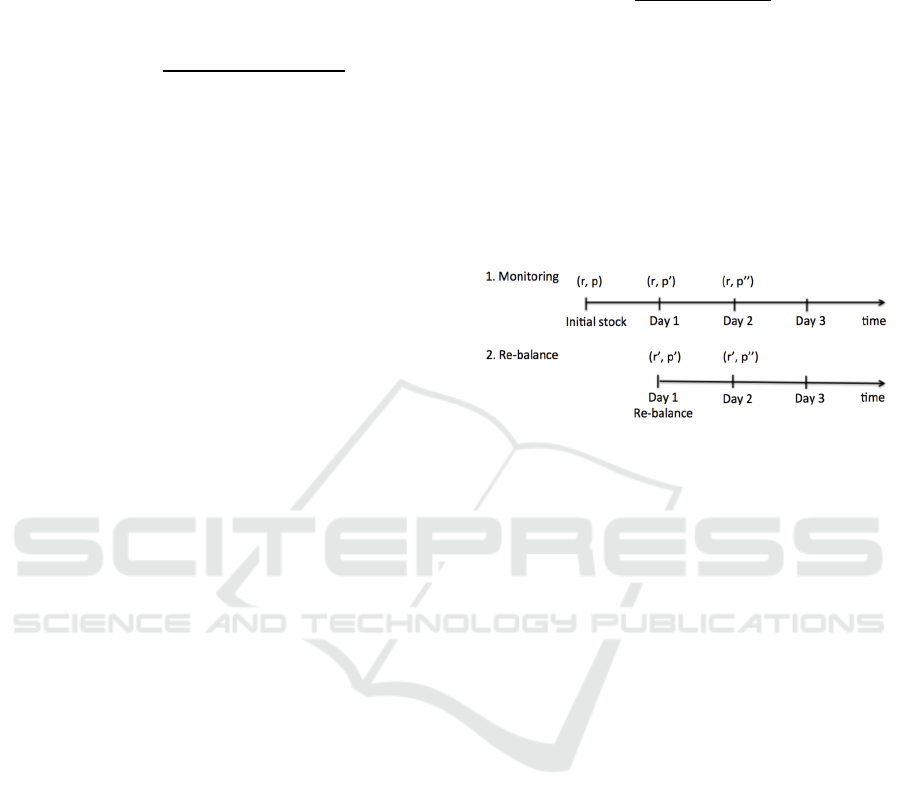
3.3 Inventory Stock Re-balance
For some merchandises, if the inventory can be
replenished or adjusted among warehouses, knowing
the actual p'(i) at the end of day 1, we can update the
warehouse allocation ratio for the SKU in region i
using
∗′
∑
∗′
(3)
where p
'
i
p
i
|
r
i
is the newly observed sales
conversion rate given warehouse allocation according
to r(i). With the above p'(i) measurement values, it
yields a new inventory allocation ratio for the SKU as
r’
1
0,r’
2
93%andr’
3
7%
If we can re-balance the inventory among warehouses
according to the new values, our overall conversion
rate expectation for the SKU will be p" =
∑
r'
i
*p'i
= 85% based on the new sales rate data.
Figure 3: Monitoring and updates over time.
It is noted that the inventory monitoring and replenish
strategy discussed here are not something new.
Similar computations can be found in various
Bayesian applications and in general literature (Pearl,
1994).
3.4 Relationship with the ML Models
The Bayesian Updating strategy can be very useful
for flash sale regional warehouse pre-allocation with
limited inventory if we do not have an accurate
estimate of either sales proportion rate or allocation
ratio for major portion of the merchandises. The
GBDT_SCR model prediction can be used with prior
information to compute the warehouse allocation
ratio in the Bayesian Updating computation.
It is noted that if the sales conversion estimation
is accurate and consistent, meaning p'(i) = p(i),
Bayesian Updating generates the same allocation
result as before.
4 CONCLUSIONS
In flash sale, business usually acquires sufficient
quantity of merchandises that are aimed to sell out in
every sales event. We can design a merchandise
allocation robot for regional warehouses knowing
total available quantity of a SKU before the sales
event starts. The robot comprises of two components,
Bayesian Inventory Planning with Imperfect Demand Estimation in Online Flash Sale
347

a ML model prediction that computes a SKU’s
regional allocation ratio and sales conversion
probability, and a Bayesian Updating allocation
calculator that utilizes ML sales conversion model
prediction with known allocation prior. We showed
that we can forecast, monitor and improve overall
sales conversion rate progressively.
The effectiveness of the two components is
summarized in Table 2.
Table 2: Model Effectiveness.
GBDT Model Bayesian
Updating
SKUs with
repeated or
large quantity
sales
GBDT_ALR
has low
variance, higher
precision
If prediction is
accurate, trivial
operation, no or
less effect
SKUs with
shallow
quantity, short
or no past sales
GBDT_ALR
has high
variance, noisy
and lower
precision
Use
GBDT_SCR
with prior, more
effective
ACKNOWLEDGEMENTS
We thank vip.com for the continuous support.
REFERENCES
O'Sullivan, A. and Sheffrin, S., 2005. Economics:
Principles in Action. Prentice Hall.
DeGroot, M. and Schervish, M., 2002. Probability and
Statistics (third ed.). Addison-Wesley.
Savino, J., 2011. Inventory to Support Flash Sales
Environments, MultiChannel Merchant (available at
http://multichannelmerchant.com/opsandfulfillment/inv
entory-to-support-flash-sales-environments-02022011/).
Ghiani, G., Laporte G., Musmanno R., 2004. Introduction
to Logistics Systems Planning and Control. John Wiley
& Sons.
Stevenson, W. J., 2009. Operations Management (10th
edition). McGraw-Hill Education.
Malakooti, Behnam, 2013. Operations and Production
Systems with Multiple Objectives. John Wiley & Sons.
Edgeworth, F., 1888. The Mathematical Theory of
Banking. J. Royal Statistical Society. 51,113-127.
Arrow, K., Harris, T., Marshak, J., 1951. Optimal Inventory
Policy, Econometrica.
Gallego, G. and I. Moon, 1993. The Distribution Free
Newsboy Problem: Review and Extensions. Journal of
Operational Research Society. 44, 825-834.
Friedman, J., 1999. Greedy Function Approximation: A
Gradient Boosting Machine. (available at http://www-
stat.stanford.edu/~jhf/ftp/trebst.pdf)
Hau L. Lee, V. Padmanabhan, and Seungjin Whang, 1997.
Information distortion in a supply chain: The bullwhip
effect. Mangement Science, 43(4):546–558, Apr. 1997.
Gelman, A., Carlin, J., Stern, H., Rubin, D., 2003. Bayesian
Data Analysis, Chapman and Hall/CRC, 2
nd
edition.
Pearl, J., 1994. A probablistic calculus of actions.
Proceedings of the Tenth Conference on Uncertainty in
Artificial Intelligence, Seattle. Morgan Kaufmann,
454–462.
ICORES 2016 - 5th International Conference on Operations Research and Enterprise Systems
348
