
On the Computation of the Number of Bubbles and Tunnels of a
3-D Binary Object
Humberto Sossa
Instituto Politécnico Nacional-CIC, Av. Juan de Dios Bátiz S/N, Gustavo A Madero 07738, Mexico City, Mexico
Keywords: 3-D Binary Object, Number of Voids or Bubbles of a 3-D Object, Number of Tunnels of a 3-D Object.
Abstract: Two formulations and two general procedures useful to compute the number of bubbles and tunnels of 3-D
binary objects are introduced in this paper. The first formulation is useful to compute the number of bubbles
or voids of the object, while the second one is only useful to compute the number of tunnels or holes of the
object. The first procedure allows obtaining, in two steps, the number of bubbles and tunnels of a 3-D object.
Finally, the second procedure permits computing, in three steps, the number of bubbles and tunnels of several
3-D objects from an image containing them. Correctness of the functioning of the two formulations is
established theoretically. Results with a set of images are provided to demonstrate the utility and validity of
the second proposed procedures.
1 INTRODUCTION
Determining the number of bubbles (voids or
cavities) and tunnels (holes) of a 3-D object is an
important problem in image analysis. It can help, for
example, in the: 1) analysis of 3-D microstructures of
human trabecular bones in relation to its mechanical
properties (Uchiyama, 1999), 2) quantitative
morphology and network representation of soil pore
structure (Vogel, 2001), 3) unambiguous
classification of complex microstructures by their
three-dimensional parameters applied to graphite in
cast iron (Velichko, 2008), and 4) analysis of the
connectivity of the trabecular bone in identifying the
deterioration of the bone structure (Roque, 2009).
In this paper we first introduce two mathematical
expressions that allow computing, separately, the
number of bubbles (voids) and tunnels (holes) of a 3-
D object. Second, we describe two general methods.
The first method allows determining, in two steps, the
number of bubbles and tunnels of a 3-D object with
both cavities and holes. The second method, permits,
in three steps, to accomplish the same task but for
several objects into the same image.
The rest of the paper is organized as follows. In
section 2, several related methods to compute the
Euler number of a digital 3-D image (object) are
described. Next, in Section 3, several basic
definitions that will facilitate the reading of the paper
will be provided. After that, in Section 4, the
proposed two expressions will be presented and
demonstrated. In this same section the proposed
methods to determine the number of bubbles and
holes of 3-D objects will be described. Section 5 will
be devoted to present several examples to show the
functioning and applicability of the proposals. In
short, Section 6 will be focused to show present the
conclusions and directions for further research
concerning this investigation.
2 RELATED WORK
One way to compute the number of bubbles and
tunnels of a 3-D object could be by first computing its
Euler number. In 3-D, the Euler number establishes
the relation between the number of its bubbles and
tunnels of the object. One expression that can be used
for this goal could be the following general
formulation (Lin, 2008):
1
(1)
where
is the number of tunnels or holes of the
object and
is its number of bubbles, cavities or
voids (Lee, 1991 and Lee, 1993).
Equation (1) is the simplification of the more
general formulation:
(2)
where
represents the number of objects in a 3-D
Sossa, H.
On the Computation of the Number of Bubbles and Tunnels of a 3-D Binary Object.
DOI: 10.5220/0005629800170023
In Proceedings of the 5th International Conference on Pattern Recognition Applications and Methods (ICPRAM 2016), pages 17-23
ISBN: 978-989-758-173-1
Copyright
c
2016 by SCITEPRESS – Science and Technology Publications, Lda. All rights reserved
17

binary image. The first term of the right part of Eq.
(1) equals 1 due to
1.
One first problem with Eq. (1) is that the numbers
and
cannot be obtained by computing local
features of the 3-D object such as the number of
vertices and edges. In other words, its computation
cannot be broken into subtasks. This means that Eq.
(1) cannot be used to compute local measures.
A second problem with Eq. (1) is that both
numbers
and
are part of the same equation.
Thus, these two numbers cannot be computed directly
from Eq. (1).
In fact, observe that if a 3-D object possesses
bubbles and tunnels at the same time, number
will
add up a 1 to Eq. (1) for each bubble found; in the
other hand, number
will subtract a 1 to Eq. (1) for
each tunnel found. Thus, a 3-D object with exactly the
same number of bubbles and the same number of
tunnels will not alter the Euler number of the object.
In this case, Eq. (1) will produce a 1, due to
will cancel each other.
Different methods to compute the Euler number
of a 3-D digital object (image) have been reported in
literature. One of the first methods to accomplish this
was reported in (Gray, 1970) and (Park, 1971), but it
was only applicable for 6-connectivity. In (Kong,
1989), authors report several methods to compute the
Euler number of a discrete digital image in both 2-D
and 3-D.
In (Lee, 1987), the authors study the 3-D surface
Euler number of a polyhedron based on the Gauss-
Bonnet theorem of differential geometry.
In (Bonnassie, 2001), authors propose a method to
compute the Euler feature of a 3-D object based on
the analysis of its 3-D skeleton. The main idea is to
analyse a local interest region around each point in
the object skeleton.
In (Toriwaki, 2002), authors present several
fundamental properties of the topological structure of
a 3-D digitized picture including the concept of
neighbourhood and connectivity among volume cells
(voxels) of 3-D digitized binary pictures defined on a
cubic grid. They also introduce the concept of
simplicial decomposition of a 3-D digitized object.
Following this, the authors present two algorithms for
calculating the Euler number (genus) of a 3-D figure.
In (Schladitz, 2006), authors combine integral and
digital geometry to develop a method for efficient
simultaneous calculation of the intrinsic volumes of
sets observed in binary images including surface area,
integral of mean curvature, and Euler number. To
make this rigorous, the concepts of discretization with
respect to an adjacency system and complementarity
of adjacency systems are introduced.
In (Saha, 1995), authors introduce an approach to
computing the Euler characteristic of a three
dimensional digital image by computing the change
in numbers of black components, tunnels and cavities
in a 333 neighbourhood of an object (black)
point due to its deletion.
In short in (Lin, 2008), authors describe a method
to compute the Euler feature of a 3-D image based on
two definitions of foreground run and neighbour
number.
3 DEFINITIONS
In order for the reader to understand the idea behind
the proposal, several concepts are next defined. Such
concepts are helpful to derive and prove the formal
propositions that govern the operation of the proposed
methods to compute the number bubbles and tunnels
of 3-D objects.
Definition 1 (voxel). In a regular grid in three-
dimensional space, a voxel is the cubic unit that
makes part of a 3-D object. It is the minimal
processing unit in a 3-D matrix.
Definition 2 (voxel connectivity). Let
and
be two object voxels as specified in Definition 1. If
and
share a face, then it is said that both voxels
are face connected; otherwise, if
and
are
connected by one of their edges or corners, then they
are connected by an edge or by a corner; else,
and
are said to be connected at all.
Figure 1: (a) Two face connected voxels. (b) Two voxels
connected by an edge. (c) Two voxels connected by a
corner. (d) The not connected voxels.
Figure 1 shows the prior four cases given in
Definition 2 as follows: In Fig. 1(a) the two voxels
are face connected; in Fig. 1(b) the two voxels are
edge connected; in Fig. 1(c) the two voxels are corner
connected; in Fig. 1(d) the two voxels are not
connected. In this paper we will consider as
interesting objects those composed of face-connected
voxels. This suggest the following definition:
Definition 3. A connected 3-D object composed
of voxels,
is any connected set of voxels
connected only by their faces.
ICPRAM 2016 - International Conference on Pattern Recognition Applications and Methods
18
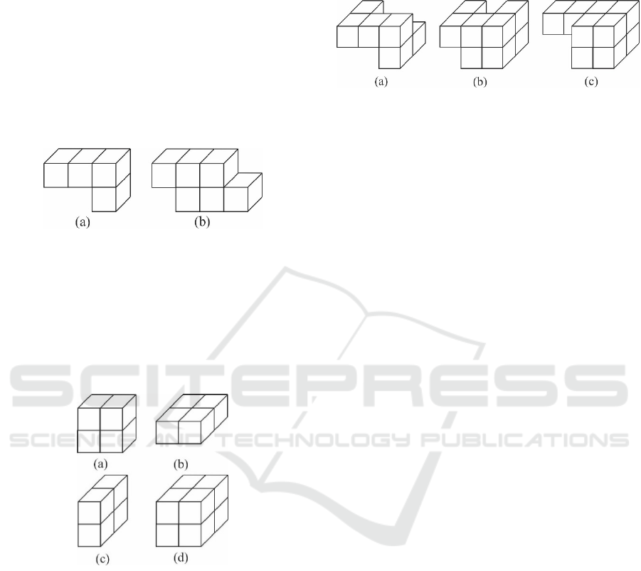
Figures 2(a) and 2(b) show two face connected
objects composed, of four and six voxels,
respectively.
Definition 4. Let
a face-connected 3-D as
stipulated by Definition 2. The faces common to the
pixels of
(the faces that interconnect the
pixels) will be called contact faces. The remaining
faces will be called exterior faces due to they connect
some of the object voxels to the background.
For example, the face connected object depicted
in Fig. 2(a) possesses four contact faces and 18
exterior faces.
Figure 2: (a) Object composed of four face connected
voxels; (b) object composed of six face connected voxels.
Definition 5. Let
be an object composed of
face connected voxels. A tetra-voxel is an
arrangement of four object voxels as shown in Fig.
3(a), 3(b) or 3(c). Let be the number of tetra-voxels
that can be found in a 3-D binary image by a simple
scanning image method.
Figure 3: A tetra-voxel in the (a) , (b) and (c) direction,
respectively. (d) An octo-voxel.
Definition 6. Let
be an object composed of
face connected voxels. An octo-voxel is an
arrangement of eight object voxels as shown in Fig.
3(d). Let be the number of octo-voxels that can be
found in a 3-D binary image by a simple scanning
image method.
To better understand these two last definitions, let
us consider the following three objects shown in Fig.
4, composed of 6, 9 and 10 voxels, respectively. After
scanning the first object, we observe that no tetra-
voxels or octo-voxels can be found. After scanning
the second object, we note that it contains two tetra-
voxels, one in the direction and one in the
direction. Finally, after scanning the third object, we
appreciate that it contains an octo-voxel and six tetra-
voxels).
Figure 4: (a) An object with no tetra-voxels or octo-voxels;
(b) An object with two tetra-voxels, one in the direction
and one in direction; (c) An object with one octo-voxel and
six tetra-voxels.
4 THE PROPOSAL
Let
a 3-D object composed of face connected
voxels for which we want to determine its number of
bubbles and it number of tunnels. Let , and ,
the number of the contact faces, number of tetra-
voxels, and number of octo-voxels of
,
respectively.
4.1 Number of Bubbles of a 3-D Object
Suppose we want to compute the number of bubbles
of an object
with no tunnels. For this we propose
to use the following:
Proposition 1. For a connected 3-D binary object:
, composed of voxels, its number of bubbles
(voids) is always given as:
1
(3)
Proof. The proof proceeds by mathematical
induction on the number of voxels of
. For the base
case,
consists of a single voxel. Therefore, we
have 0, values which satisfy Eq.
(3).
For the induction step, let us assume that Eq. (3)
holds for
. Let ´, ´, and ´ be the number of
contact faces, number of tetra-voxels and number of
octo-voxels, respectively, of object
that is
obtained by adding one voxel to
.
Let , and be the corresponding
numbers for this new voxel. We have that:
´
(4)
´
(5)
´
(6)
It must be shown that Eq. (3) holds for
, i.e.
´
1 ´ ´ ´
1
(7)
But this equation can be rewritten as follows:
On the Computation of the Number of Bubbles and Tunnels of a 3-D Binary Object
19

´
1
1
1 1.
(8)
This equation simplifies to:
´ 1
(9)
which we know is true.
Figure 5: (a) Object composed of 25 voxels with no
bubbles. (b) Object with one bubble after appending a voxel
to the object shown in Fig. 5(a).
To numerically validate this last equation, let us
consider the 3-D object composed of 25 voxels as
shown in Figure 5(a), with no bubbles and with the
central voxel and the central voxel from the right face
missing. For this object,
25 44 20
10 bubbles. Now, suppose that a new voxel is
appended to this object as shown in Fig. 5(b) in such
a way that a bubble is obtained. In this case we have
that 4, 4, 0, and
´
1 ´ ´ ´
1
26 48 24 0
11.
Also
´ 1 0 4
4011.
4.2 Number of Tunnels of a 3-D Object
Suppose now we want to compute the number of
tunnels of an object
with no bubbles. For this we
propose to use the following:
Proposition 2. For a connected 3-D binary object:
, composed of voxels, its number of tunnels
(holes) is always given as:
1
(10)
Proof. Let us again proceed with the proof by
mathematical induction on the number of voxels of
. For the base case,
consists of a single voxel.
Therefore, we have 0, values which
satisfy Eq. (10).
For the induction step, let us assume that Eq. (10)
holds for
. Let ´, ´, and ´ be the number of
contact faces, number of tetra-voxels and number of
octo-voxels, respectively, of object
that is
obtained by adding one voxel to
.
Let , and be the corresponding
numbers of this new voxel. We have that:
´
(11)
´
(12)
´
(13)
It must be shown that Eq. (10) holds for
, i.e.
´ 1
1 ´ ´ ´
(14)
But this equation can be rewritten as follows:
´ 1
1
1
1.
(15)
This equation simplifies to:
´ 1
(16)
which again we know is true.
To numerically validate this last equation, let us
consider the 3-D object composed of 6 voxels as
shown in Fig. 6(a), with no tunnels. For this object,
1
760
0 tunnels. Now, suppose
that a new voxel is appended to this object as shown
in Fig. 6(b) in such a way that a tunnel is obtained. In
this case we have that 2, 0, 0, and
´ 1
1 ´ ´ ´
1
8800
1.
Also
´ 1 0 2
0011.
Figure 6: (a) Object composed of 7 voxels with no tunnels.
(b) Object with one tunnel after appending a voxel to the
object shown in Fig. 6(a).
4.3 Computing the Number of Bubbles
and Tunnels of a 3-D Object
Suppose now we want to compute the number of
bubbles and tunnels of an object
that might have
several of them in it. To accomplish this task we
proceed in two steps. During the first step we obtain
the number of bubbles of the object. For this, we make
use of a connected component labelling algorithm.
During the second step we obtain its number of
ICPRAM 2016 - International Conference on Pattern Recognition Applications and Methods
20
tunnels by using Eq. (10). More in detail, given a 3-D
image of object
:
First step (Number of bubbles):
1. Apply over any connected component
algorithm over the regions composed of 0-voxels.
An adapted version of the algorithm reported in
(Gonzalez, 2002) can be used for this goal. Due to
bubbles are composed of 0-voxels, this algorithm
will output value . This variable corresponds
to the number of bubbles plus 1. This 1 is obtained
because the image background was also labelled;
an extra label was generated.
2. Compute the number of bubbles of the object,
as 1.
Second step (Number of tunnels):
1. Apply Eq. (10) over image . If the object has
bubbles and tunnels, this application will produce
the number of tunnels minus the number of
bubbles, _. Refer to Eq. (1).
2. Add to the result obtained in the last step to get the
number of tunnels _ of object
.
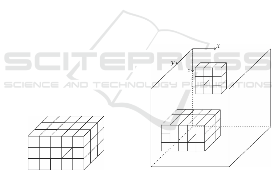
To numerically validate the above described
procedure, let us consider the object shown in Figure
7, composed of 41 voxels, one bubble and one tunnel.
The bubble is the 0-voxel in the centre of the second
slice of 1-voxels of the object (left to right). The
tunnel is composed of the three 0-voxels along the
fourth slice of 1-voxels of the object (left to right).
The first step outputs 1, while the second
step outputs _ 1
41 76
36 0
101, as desired. Note that _ 0
due to the object has one bubble and one tunnel, that
according to Eq. (1) they cancel each other.
Figure 7: Object composed of 41 voxels used to test the
functioning of the described procedure.
4.4 Computing the Number of Bubbles
and Tunnels of a Set of 3-D Objects
Suppose now are given an image of
voxelized
objects; for each of these
we would like to compute
their numbers of bubbles and tunnels, respectively. In
this case we would need to apply a similar procedure
as described in section 4.3 with an additional step. We
proceed into three steps as follows:
During the first step, we apply any connected
component algorithm over image . As a result we
obtain
labelled connected 3-D regions.
During the second step we apply the first step of
the procedure described in section 3.3 to each labelled
connected region
, 1,2,…,
. For each
we
obtain its number of bubbles
, 1,2…,
.
Finally, for the third step we apply the second step
of the same procedure described in section 3.3 to
obtain the number of tunnels of each object.
To numerically validate the above described
procedure, let us consider Fig. 8 with two objects; the
first one composed of 8 voxels and one tunnel and the
second one integrated of 41 voxels, with one bubble
and one tunnel (the same object of Fig. 7).
The first step provides as a result two labels (two
connected 3-D regions). Now, for each label (region),
the second step obtains
0 and
1,
respectively. Finally, the third step outputs
_
1
8800
010
1 for the first object and
_
1
41 76 36 0
1011, for the
second object, as desired.
Figure 8: Image with two object used to show the
functioning of the described procedure.
5 RESULTS
In this section we report four experiments. First we
verify the correct functioning of the proposal with a
set of five 3-D images of size 100 100 100
voxels. Each image has a different number of objects
with a different increasing number of voxels, as
On the Computation of the Number of Bubbles and Tunnels of a 3-D Binary Object
21
established in row two of Table 1. Each time an object
was added to the image it was added manually to have
a control over the number of bubbles and holes. Rows
3 and 4 of Table 1 show the correct number of bubbles
and tunnels (Correct and Correct ) of each
object of each image, respectively.
Table 1: Results obtained by the application of the
procedure to the five selected objects.
Image number 1 2 3 4 5
Number of
objects
1 2 3 4 5
Correct
2 2,1 2,1,3 2,1,3,2 2,1,3,2,5
Correct
1 1,3 1,3,1 1,3,1,2 1,3,1,2,4
Computed
2 2.1 2,1,3 2,1,3,2 2,1,3,2,5
Computed
1 1,3 1,3,1 1,3,1,2 1,3,1,2,4
The procedure described in section 4.4 was
applied to each of the five images. It was programed
in Java NetBeans with the Processing Applet in a
desktop computer with a Core i7 model 2600
processor with 8Gb of RAM. Rows 5 and 6 depict the
computed number of bubbles and tunnels for object
of each image, respectively. From these rows note
also that in all cases, as expected, the correct values,
and , for each object were produced by the
procedure. The average time to compute the number
of bubbles and tunnels of each of the
objects in
image was 29.6 milliseconds. It is worth
mentioning that most of time is consumed by the
connected component algorithms.
Second, we studied if the number of object-voxels
influenced computation time when the total
procedure was applied over an image. For this, we
automatically generated a set of images with an
increasing number of object-voxels. We established a
variable () defining how many object-voxels will
appear in the image. When 0.0, it meant that the
corresponding image will have only background
voxels, for 0.05, it meant that 5% of the
generated voxels will belong to objects, and so on.
Each time we increased variable by 0.05. For each
value of variable we generated 10 images. We
took the average time to fully process the whole set
of 210 images and computed the average time. With
the exception of the first case, in average this time
consumed by the connected component algorithm
was of 25.5 milliseconds.
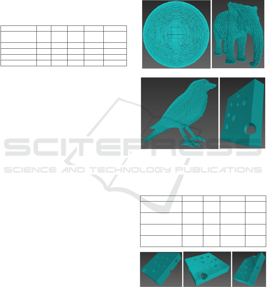
Third, we demonstrated the applicability of our
method when applied to objects of various shapes and
complexities. Figure 9 show four of these objects: a
sphere, an elephant, a bird and a cheese. In all cases
images of 120 120 120 voxels were used.
Second and third row of Table 2 show the true values
of number of bubbles and tunnels of each object while
fourth and fifth rows show the computed values. As
expected it can be seen that in all four cases, the
computed values coincide with the true values. The
average time to obtain the desired results was of 51.8
milliseconds.
(a) (b)
(c) (d)
Figure 9: Four objects of different shape and complexities
to demonstrate the applicability of the proposal.
Table 2: Results obtained by the application of the
procedure to the four objects of Figure 9.
Object Sphere Bird Elephant Cheese
Correct number of
bubbles
0 0 0 0
Correct number of
tunnels
0 0 0 10
Computed number
of bubbles
0 0 0 0
Computed number
of tunnels
0 0 0 10
Figure 10: Three transformed versions of cheese objects.
Finally, we showed the robustness of our method
to image transformations such as translations,
rotations and scale changes. For this, we took the
cheese object and translated, rotated and scaled inside
ICPRAM 2016 - International Conference on Pattern Recognition Applications and Methods
22

its image. Three of these transformed versions are
depicted in Figure 10. Again, in all cases, the desired
number of tunnels: 10 was correctly computed.
6 CONCLUSIONS AND
FURTHER RESEARCH
From the theoretical point of view, we have
introduced two formulations ((Eq. (3) and Eq. (10))
that allow determining the number of bubbles and
tunnels, respectively, of any 3-D binary face
connected object in an exact way. Both equations
have been mathematically demonstrated; numerical
examples have also been provided to numerically
validate both equations.
From the practical point of view, we have
presented two procedures. The first procedure,
described in detail in section 4.3, permits determining
the number of bubbles and tunnels of a 3-D binary
face connected object from a binary image of it. The
second general procedure, fully explained in section
4.4, allows to do the same but for several objects.
Experimental results with images of object of
different sizes and complexities have been given to
show the applicability of both procedures.
The time spent in seconds expended by the
proposal is reduced making the procedure to be used
in real time applications.
Further work in this direction include:
Implementation of the proposed general procedure
described in section 4.4 into a FPGA or a GPU
processor to see how much the processing time could
be reduced. This will be of particular interest when
processing large images with many objects in them.
ACKNOWLEDGEMENTS
Humberto Sossa would like to thank COFAA-IPN,
SIP-IPN and CONACYT under Grants 20151187,
155014 and 65 (Frontiers of Science), respectively,
for the economic support to carry out this research.
REFERENCES
Uchiyama, T. et al., 1999. Three-Dimensional
Microstructural Analysis of Human Trabecular Bone in
Relation to Its Mechanical Properties. Bone 25(4):487–
491.
Vogel, HJ. and Roth, K., 2001. Quantitative morphology
and network representation of soil pore structure.
Advances in Water Resources 24:233-242.
Velichko, A. et al., 2008. Unambiguous classification of
complex microstructures by their three-dimensional
parameters applied to graphite in cast iron. Acta
Materialia 56:1981-1990.
Roque, WL. et al., 2009. The Euler-Poincaré characteristic
applied to identify low bone density from vertebral
tomographic images. Rev Bras Reumatol 49(2):140-52.
Lin, X. et al., 2008. A New Approach to Compute the Euler
Number of 3D Image. In 3rd IEEE Conference on
Industrial Electronics and Applications, pp. 1543-
1546.
Lee, CN. et al., 1991. Winding and Euler numbers for 2D
and 3D digital images, CVGIP: Graph. Models Image
Process, 53(6):522-537.
Lee, CN. et al. 1993. Holes and Genus of 2D and 3D digital
images, CVGIP: Graph. Models Image Process,
55(1):20-47.
Gray, SB., 1970. Local Properties of Binary Images in Two
and Three Dimensions, Boston: Information
International Inc.
Park, CM. and Rosenfeld, A., 1971, Connectivity and
Genus in Three Dimension, TR-156, Computer Vision
Laboratory, Computer Science Center, University of
Maryland, College Park, MD.
Kong, TY. and Rosenfeld, A., 1987. Digital Topology:
Introduction and Survey, Computer vision Graphic and
Image Processing, 48:357-393.
Lee, CN. and Rosenfeld, A., 1987. Computing the Euler
Number of a 3D Image, In Proceedings of the IEEE
First International Conference on Computer Vision, pp.
567-571.
Bonnassie, A. et al., 2001. Shape description of three-
dimensional images based on medial axis. In
Proceedings of the 2001 International Conference on
Image Processing, pp. 931-934.
Toriwaki, J. and Yonekura, T., 2002. Euler Number and
Connectivity Indexes of a Three Dimensional Digital
Picture. Forma, 17:183–209.
Schladitz, K. et al., 2006. Measuring Intrinsic Volumes in
Digital 3D Images. A. Kuba, L.G. Nyúl, and K. Palágyi
(Eds.): In DGCI 2006, LNCS 4245, pp. 247–258.
Saha, PK. and Chaudhuri, BB., 1995. A new approach to
computing the Euler Characteristic. Pattern
Recognition 28(12):1955-1963.
Gonzalez, R. and Woods, R., 2002. Digital Image
Processing. Prentice Hall.
On the Computation of the Number of Bubbles and Tunnels of a 3-D Binary Object
23
