
Statistical Measurement Validation with Application to Electronic Nose
Technology
Mina Mirshahi, Vahid Partovi Nia and Luc Adjengue
Department of Mathematics and Industrial Engineering, Polytechnique Montreal, Montreal, Quebec, Canada
Keywords:
Artificial Olfaction, Electronic Nose, Gas Sensor, Odor, Outlier, Robust Covariance Estimation.
Abstract:
An artificial olfaction called electronic nose (e-nose) relies on an array of gas sensors with the capability of
mimicking the human sense of smell. Applying an appropriate pattern recognition on the sensor’s output
returns odor concentration and odor classification. Odor concentration plays a key role in analyzing odors.
Assuring the validity of measurements in each stage of sampling is a critical issue in sampling odors. An ac-
curate prediction for odor concentration demands for careful monitoring of the gas sensor array measurements
through time. The existing e-noses capture all odor changes in its environment with possibly varying range of
error. Consequently, some measurements may distort the pattern recognition results. We explore e-nose data
and provide a statistical algorithm to assess the data validity. Our online algorithm is computationally efficient
and treats data as being sampled.
1 INTRODUCTION
The ability to recognize the chemicals in the envi-
ronment is a very basic and essential need for the
living organisms; from a single-cell amoebae to hu-
man beings, all species are provided with a chemi-
cal awareness system. Human beings have three sen-
sory systems to detect odors: sense of taste, sense of
smell, and chemical feel with receptors all over the
body. All species employ their chemical senses to
approach and being attracted to possibly safe condi-
tions, as well as avoiding and being resisted to the
harmful ones. As for human beings, in every breath,
the sense of smell collects a sample from its environ-
ment and forwards it to the brain for further analyses.
Unlike the sense of taste, smell can be captured from
a distance and assist the brain in producing a warn-
ing. Unfortunately, the human sense of smell does
not respond to all harmful air pollutants. Additionally,
sensitivity of humans to many air pollutants varies —
one can be accustomed to a toxic smell. In the last
decade, great attention has been paid to the subject
of air quality because it directly influences the envi-
ronmental and human health. A crucial element in
assessment of indoor and outdoor air quality is audit-
ing the odorants. There exists various odor measure-
ment techniques such as dilution-to-threshold, olfac-
tometers, and referencing techniques (McGinley and
Inc, 2002). The performance of these approaches de-
pend on human evaluation. Due to the high variabil-
ity of individual’s sensitivity, the common methods
mostly lack accuracy. In 1982, the first gas multi-
sensor array was invented as primary artificial olfac-
tion (Persaud and Dodd, 1982). The term electronic
nose (e-nose) was introduced by Gardner and Bartlett
(1994). E-nose is an artificial olfactory system which
consists of an array of gas sensors. The e-nose is
designed for recognizing complex odors in its sur-
rounding environment. The gas sensor array receives
chemical information about gaseous mixtures as in-
put and converts it to measurable signals. Sensors
act independently and simultaneously in this device.
Cross-sensitivity of gas sensors is inevitable in sen-
sor array structure. The cross-sensitivity is the inter-
action among chemicals that leads to a different sig-
nal from the component in a mixture compared to the
single component. Gas sensor’s performance is af-
fected by different elements which make it unstable
and less sensitive to odors. One of the most serious
deterioration in sensors is owing to a phenomenon
called drift. Drift is a temporal change in sensor’s
response while all other external conditions are kept
constant. The majority of manufactured sensor ar-
rays are subject to drift, and several methods have
been introduced to overcome this problem (Carlo and
Falasconi, 2012; Artursson et al., 2000; Padilla et al.,
2010; Zuppa et al., 2007). The behavior of a sensor is
directly influenced by the surrounding chemical and
Mirshahi, M., Nia, V. and Adjengue, L.
Statistical Measurement Validation with Application to Electronic Nose Technology.
DOI: 10.5220/0005628204070414
In Proceedings of the 5th International Conference on Pattern Recognition Applications and Methods (ICPRAM 2016), pages 407-414
ISBN: 978-989-758-173-1
Copyright
c
2016 by SCITEPRESS – Science and Technology Publications, Lda. All rights reserved
407
physical conditions. For instance, the sensor response
may depend on the temperature of the gas under ex-
amination. Therefore, thermal conditions around the
sensing elements need to be supervised. The multi-
variate response of gas sensor arrays undergoes dif-
ferent pre-processing procedures before the predic-
tion is performed using statistical tools such as regres-
sion, classification, or clustering. Numerous methods
have been developed for analyzing the gas sensor ar-
ray data, including Gutierrez-Osuna (2002); Kermiti
and Tomic (2003); Bermak et al. (2006).
2 PROBLEM STATEMENT
The e-nose has partially addressed the human sense of
smell in diverse industrial sites. Unwanted variabil-
ity may occur in sensor’s output data. This happens
due to environmental factors or physical impairment
of the system, since e-noses are installed in outdoor
fields where the conditions can dramatically fluctu-
ate. This demands for monitoring the critical factors
through adding extra sensors and temperature com-
pensation in sensor pre-processing. The sensor’s out-
put is used to quantify odor concentration. Transfer-
ring the data to olfactometry is both time consuming
and costly. Only small portions of data are appointed
for further analyses of its concentration in olfactom-
etry. Pattern recognition methods are employed in
order to predict the odor concentration for each set
of sensor values. To assess the accuracy of predic-
tions, the validity of sensor values must be ensured.
Sensors in the e-nose structure may report incorrect
values or some stop functioning for a short period of
time. These anomalies are ought to be diagnosed and
reported in real time using a computationally efficient
algorithm.
3 DATA DESCRIPTION
The data under the study include 11 distinct attributes,
each representing sensor values of the e-nose. Sen-
sors react to almost all gases in the air, but they are
designed so that each sensor is more sensitive to a
specific type of gas. Some of the sensors are highly
positively correlated with each other, see Figure 1 and
Figure 2 (left panel).
Suppose that x
>
p×1
is a random vector of p = 11 at-
tributes, in which a
>
illustrates the transpose of vector
a, and its n independent realization are stored in the
rows of data matrix X
n×p
. The covariance matrix of
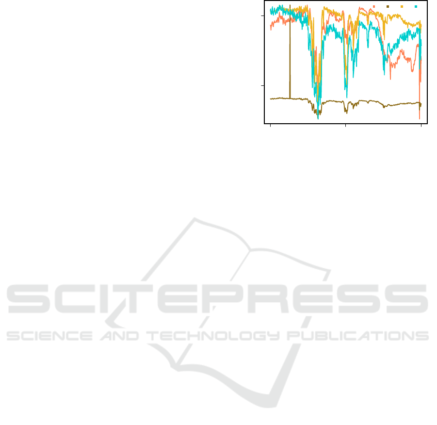
Time
Sensor’s Output × 10
4
Jan−28 Jan−29 Jan−30
5.1 5.2
s
1
s
2
s
5
s
8
Figure 1: Senor’s output during three days of sampling for
4 randomly selected sensors.
x
p×1
, say Σ = [σ
i j
]
i, j=1,2,..., p
, is defined as
Σ
p×p
= Cov(x) = E{(x − µ)(x − µ)
>
},
where µ represents the mean of x, E is the expecta-
tion operator. The covariance, σ
i j
, measures the de-
gree to which two attributes are linearly associated. It
is well-known that the inverse of covariance matrix,
commonly known as precision matrix, yields the par-
tial correlation between the attributes. The partial cor-
relation is the correlation between two attributes con-
ditioning on the effect of other attributes. Non-zero
elements of Σ
−1
implies the conditional dependence.
Therefore, the sparse estimation of Σ
−1
pinpoints the
block dependent structure of attributes. The sparse es-
timation of Σ
−1
set some of the Σ
−1
entries exactly
to zero. Investigation of the inherent dependence be-
tween the sensor values is then performed by means
of the partial correlation. In order to obtain a clear
image of sensors which are potentially grouped to-
gether, the graphical lasso (Friedman et al., 2008) is
used. Friedman et al. (2008) considered estimating
the inverse of covariance matrix, Σ
−1
, sparsely by
applying a lasso penalty (Tibshirani, 1996). In Fig-
ure 2 (right panel), the undirected graph connects two
variables which are conditionally correlated given all
other attributes. For instance, the sensors 9, 10, and
11 are conditionally correlated with each other. This
also agrees with the heatmap of the correlation ma-
trix Figure 2 (left panel). Thus, this dependence must
be taken into account while modeling data. Another
vital assumption that should be verified is the Gaus-
sianity of the data. The non-Gaussianity of the sensor
values is established using various methods such as
analyzing the distribution of individual sensor values,
scatter plot of the linear projection of data using prin-
cipal components, estimating the multivariate kurtosis
and skewness, and also multivariate Mardia test, see
Figure 3.
ICPRAM 2016 - International Conference on Pattern Recognition Applications and Methods
408
s
11
s
9
s
7
s
5
s
3
s
1
s
1
s
3
s
5
s
7
s
9
s
11
−1
−0.8
−0.6
−0.4
−0.2
0
0.2
0.4
0.6
0.8
1
1
2
3
4
5
6
7
8
9
10
11
Figure 2: Left panel, heatmap of the correlation matrix of the sensor values (s
1
–s
11
). Right panel, the undirected graph
of partial correlation using the graphical lasso. The undirected graph of the right panel approves the block structure of the
heatmap of the left panel.
0 200 400 600 800 1000
10 20 30 40
Squared Mahalanobis Distance
Chi−Square Quantile
× 10
−4
35 40 45 50
0246
s
1
× 10
3
Density
× 10
−4
35 40 45 50
0246
s
6
× 10
3
Density
× 10
−4
35 40 45 50
0246
s
11
× 10
3
Density
Figure 3: Left panel, the Q-Q plot of squared Mahalanobis distance supposed to follow chi-square distribution for Gaussian
data. Right panel, the marginal density for some randomly chosen sensor values. Both graphs confirm the non-Gaussianity of
data.
4 METHODOLOGY
In order to demonstrate the validity of the e-nose mea-
surements, we aim to allocate each sample to different
zones. To be able to verify the validity of the measure-
ments, it is necessary to have some reference samples
for the purpose of comparison. These reference sam-
ples are collected while the e-nose is at its best per-
formance, and the conditions are fully under control.
For the data set under the study, there are two distinct
reference sets. Reference 1 is constituted of data in a
period of sampling defined by an expert after installa-
tion of the e-nose. We call the data in this period of
sampling as proposed set. Reference 2, upon its avail-
ability, is manually gathered samples from the field
and brought to the laboratory to quantify the odor con-
centration. We call the latter data, calibration set to
emphasize that it can be used for data modeling us-
ing supervised learning. If new data diverge greatly
from the overall pattern of data previously seen, then
it is marked as an outlier and is allocated to the red
zone. This zone represents a dramatic change in the
pattern of samples and refer to “risky” samples. If
new data is non-outlier and it is also located within the
data polytope of the Reference 1 or the Reference 2, it
is assigned to green or blue zone respectively. These
zones represent the “safe” samples. If new data is
non-outlier, but outside of the area of green and blue
zones, it is assigned to yellow zone. This zone dis-
plays potentially “critical” samples.
Producing many samples belonging to the yellow
and the red zones is an indication of a major flaw in
the system. Physical complications, such as sensor
loss in the e-nose, or sudden changes in the chem-
ical pattern of the environment, account for all un-
desirable measurements. Zone assignment, therefore,
require some outlier detection algorithms. To de-
fine the green and the blue zones, the new samples
Statistical Measurement Validation with Application to Electronic Nose Technology
409
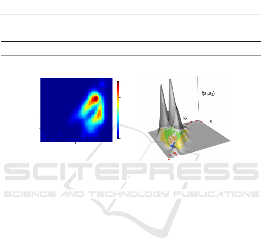
Table 1: Description of each zones in validity assessment procedure.
Zone Description
Red Observations that are outliers in terms of AO measure.
Green
Observations that are non-outliers in terms of AO measure. Moreover, they fall into the polytope
of the Reference 1.
Blue
Observations that are non-outliers in terms of AO measure. Moreover, they fall into the polytope
of the Reference 2.
Orange
Observations that are non-outliers in terms of AO measure. Moreover, they fall into the polytopes
of both the Reference 1 and the Reference 2.
Yellow
Observations that are non-outliers in terms of AO measure. Moreover, they do not fall into the
polytope of neither the Reference 1 nor the Reference 2.
44 48 52
36 37 38 39
s
1
× 10
3
s
2
× 10
3
0
0.5
1
1.5
2
× 10
−7
Figure 4: Validity assessment for about 700 samples based on 2 sensor values. Left panel, the plot illustrates the contour map
of estimated density function for the 2 sensors. Right panel, the density function of the samples demonstrated in 3D with
zones identified for each of the samples in the sensor 1 (s
1
) versus sensor 2 (s
2
) plane. Higher density is assigned to green,
blue, and orange zones compared to yellow and red zones.
are projected onto a lower dimension subspace. Di-
mension reduction methods such as principal compo-
nent analysis (PCA) can serve this purpose (Jolliffe,
2002). PCA transforms a collection of possibly corre-
lated attributes into a set of linearly uncorrelated axes
through orthogonal linear transformations. The first k
(k < p) principal components are the eigenvectors of
the covariance matrix Σ associated with the k largest
eigenvalues. PCA exploits empirical covariance ma-
trix,
ˆ
Σ, which is extremely sensitive to outliers (Pren-
dergast, 2008). Since the data contain many outliers,
robust covariance estimation must be applied to avoid
misleading results. Robust principal component anal-
ysis (Hubert et al., 2005) is employed for dimension
reduction purpose throughout this paper. This robust
PCA computes the covariance matrix through projec-
tion pursuit (Li and Chen, 1985) and minimum co-
variance determinant (Croux and Haesbroeck, 2000)
methods. The robust PCA procedure can be summa-
rized as follows:
1. The matrix of data is pre-processed such that the
data spread in the subspace of at most min(n −
1, p).
2. In the spanned subspace, the most obvious out-
liers are diagnosed and removed from data. The
covariance matrix is calculated for the remaining
data,
ˆ
Σ
0
.
3.
ˆ
Σ
0
is used to decide about the number of principal
components to be retained in the analysis, say k
0
(k
0
< p).
4. The data are projected onto the subspace spanned
by the first k
0
eigenvectors of
ˆ
Σ
0
.
5. The covariance matrix of the projected points is
estimated robustly using minimum covariance de-
terminant method and its k leading eigenvalues are
computed. The corresponding eigenvectors are
the robust principal components.
To define the red zone, it is required to find the
outliers of data as it is being measured by the e-nose
through time. As the data fail to follow a Gaussian
distribution, outlier detection methods that rely on the
assumption of elliptical contoured distribution should
be avoided. Here, outliers are flagged by means of ad-
justed outlyingness (AO) criterion (Brys et al., 2006).
If a sample is detected as an outlier by AO measure,
it belongs to the red zone. For the specification of the
ICPRAM 2016 - International Conference on Pattern Recognition Applications and Methods
410

remaining zones, we need to define the polytopes of
the samples in Reference 1 and Reference 2. These
polytopes are built using the convex hull of the ro-
bust principal component scores. More specifically,
the boundary of the green zone is defined by com-
puting the convex hull of the robust principal compo-
nent scores of the Reference 1. A short description of
each zone is provided in Table 1. Before determin-
ing the color tag for each new data, the samples are
checked for missing values and are imputed in case
needed by multivariate imputation methods such as
Josse et al. (2011). The idea behind the validity as-
sessment is visualized in Figure 4. For simplicity,
only 2 sensors are used for all computations in Fig-
ure 4 and a 2D presentation of zones is plotted using
the sensors’ coordinates. Suppose that X
N×11
repre-
sents the matrix of sensor values for N samples, y
N
the vector of corresponding odor concentration val-
ues and x
>
l
is the lth row of X
N×11
, l = 1, 2, . . . , N.
Furthermore, suppose that n
1
refers to the number of
samples in the proposed set of the sampling and n
2
refers to the number of samples in the calibration set.
The samples of the proposed set are always available,
but not necessary the calibration set. Two different
scenarios occur based on the availability of the cali-
bration set. If the calibration set is accessible, then
Scenario 1 happens. Otherwise, we only deal with
Scenario 2. Scenario 1 is a general case which is
explained more in details. The data undergo a pre-
processing stage, including imputation and outlier de-
tection, before any further analyses. Having done the
pre-processing stage, data are stored as Reference 1,
X
n
1
×11
, and Reference 2, X
n
2
×11
. The first k, e.g.
k = 2, 3, robust principal components of X
n
1
×11
are
calculated and the corresponding loading matrix is
Sub-Algorithm: (Scenario 1).
1: if the point x
>
l
, l = 1, 2, . . . , N is identified as an
outlier by AO measure then
2: x
>
l
is in red zone,
3: else if x
>
l
L
1
∈ ConvexHull
(1)
AND x
>
l
L
1
6∈
ConvexHull
(2)
then
4: x
>
l
is in green zone,
5: else if x
>
l
L
1
6∈ ConvexHull
(1)
AND x
>
l
L
1
∈
ConvexHull
(2)
then
6: x
>
l
is in blue zone,
7: else if x
>
l
L
1
∈ ConvexHull
(1)
AND x
>
l
L
1
∈
ConvexHull
(2)
then
8: x
>
l
is in orange zone,
9: else
10: x
>
l
is in yellow zone.
11: end if
denoted by L
1
. The pseudo code of two algorithms
for Scenario 1 is provided below. Scenario 2 is a spe-
cial case of Scenario 1 in which Sub-Algorithm (Sce-
nario 1) is used with ConvexHull
(2)
= ∅ that elimi-
nates the blue and the orange zones. Consequently,
there is no model for odor concentration prediction in
the Main Algorithm.
Main Algorithm: (Scenario 1).
Require: X
n
1
×11
, X
n
2
×11
, and the loading matrix L
1
using robust PCA over Reference 1, X
n
1
×11
.
1: ConvexHull
(1)
← the convex hull of the projected
values of the Reference 1, X
n
1
×11
L
1
.
2: Train a supervised learning model on Refer-
ence 2, X
n
2
×11
, and its odor concentration vector,
y
n
2
.
3: ConvexHull
(2)
← the convex hull of the projected
values of the Reference 2, X
n
2
×11
L
1
.
4: Do Sub-Algorithm for new data x
∗
.
5: Predict the odor concentration for new data x
∗
us-
ing the trained supervised learning model.
The above steps are implemented over 8 months
of data collected by the e-nose in Section 6. In order
to justify our choice of statistical techniques, the pro-
posed methodology is run over a set of simulated data
in a following section.
5 SIMULATION
To emphasize on the importance of the assump-
tions such as non-eliptical contoured distribution and
robust estimation considered in our methodology,
we examine the methodology on a set of simu-
lated data. Assume the matrix of data X
N×2
, where
x
>
l
= (x
l1
, x
l2
); l = 1, 2, . . . , N, are generated accord-
ing to the mixture of Gaussian and the Student’s t-
distributions, Figure 5 (top left panel). Ignoring the
distribution of data and seeking for any classical ap-
proach toward outlier detection, renders some ob-
servations as outliers mistakenly, Figure 5 (top right
panel). The parameters of interest, the mean vector
and the covariance matrix, need to be estimated ro-
bustly, otherwise the confidence region misrepresents
the underlying distribution. In Figure 5 (bottom left
panel), the classical confidence region is pulled to-
ward the outlier observations. On the contrary, the
robust confidence region perfectly unveil the distri-
bution of the majority of observations because of the
robust and efficient estimation of the mean and the
covariance matrix. Consequently, the classical prin-
cipal components are affected by the inefficient esti-
Statistical Measurement Validation with Application to Electronic Nose Technology
411
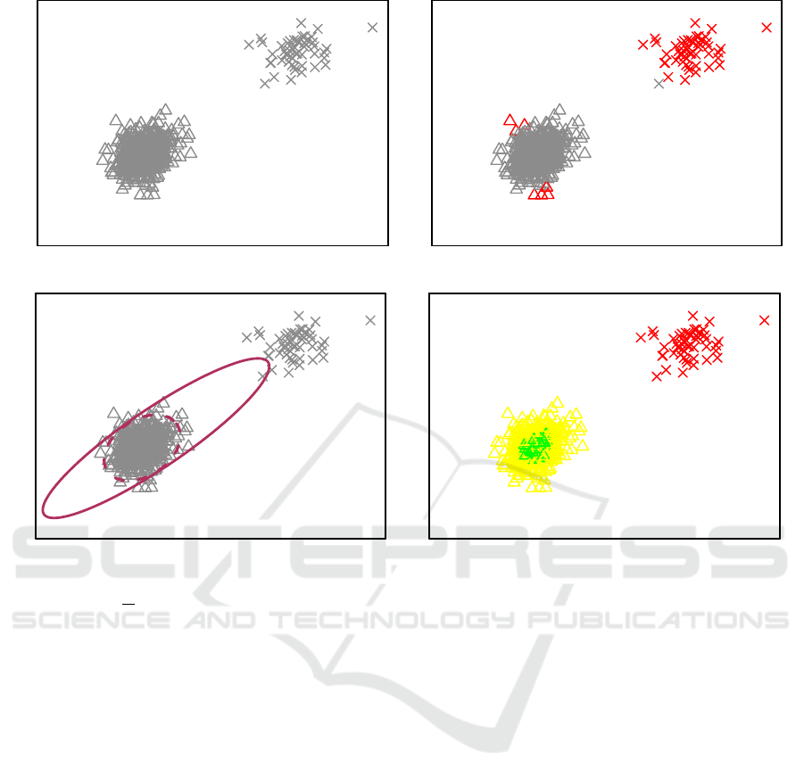
x
1
x
2
x
1
x
2
x
1
x
2
x
1
x
2
Figure 5: Top left panel, the simulated data from the mixture distribution f (x) = (1 − ε) f
1
(x) + ε f
2
(x) with contamination
proportion of ε =
1
10
, and f
1
and f
2
being the Gaussian and Student’s t-distribution respectively. The data from f
1
, and f
2
are plotted in triangles and crosses correspondingly. Top right panel, the outliers of data are identified and highlighted with
red using the classical Mahalonobis distance and 95th percentile of the Chi-square distribution with two degrees of freedom.
Bottom left panel, the 95% confidence region for the data is computed using the classical estimates of parameters (solid line)
and the robust estimates (dashed line). Bottom right panel, the Main Algorithm is implemented and the zones are graphed by
colors described in Table 1.
mation of the covariance matrix. We proposed using
methods which deal with contaminated data appropri-
ately. Adjusted outlyingness (AO) measure identifies
the outliers of the data correctly. In the Main Algo-
rithm, suppose we take the Gaussian sub-sample as
the Reference 1. Figure 5 (bottom right panel) shows
the result of our algorithm on the simulated data.
6 APPLICATION
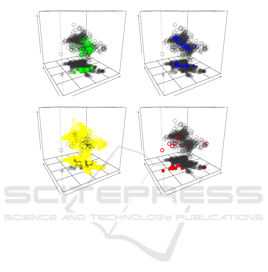
For the easy visualization, the first 3 robust princi-
ple components of the data are used, PC1, PC2, PC3.
These components correspond to the 3 largest eigen-
values of the covariance matrix. In case of sensor
failures, the data contain missing values that need to
be imputed. First, data are imputed to replace all the
missing values, and then the validity of the measure-
ments are identified over the 8 months sampling. Only
a subset of 500 samples out of 200 thousands of obser-
vations are plotted to make the graphs more readable.
In Figure 6, the sample points are drawn in gray and
each zone is highlighted using its corresponding color
of Table 1. The circles in Figure 6 are also illustrated
on PC1 and PC2 plane for a better demonstration of
the zones.
The zones’ definition is helpful in interpreting the
results. As an example, the green or the blue zone re-
veals the fact that the sampling points are very close
to the samples that have already been observed in ei-
ther Reference 1 or Reference 2. The observations in
reference sets were entirely under control, therefore,
the blue and green zones justify the validity of sam-
ples. Consequently, the prediction obtained over these
samples is expected to be more accurate. On the con-
trary, the prediction values for the points in the yel-
low zone are less accurate compared with the green
ICPRAM 2016 - International Conference on Pattern Recognition Applications and Methods
412
PC1
PC2
PC3
PC1
PC2
PC3
PC1
PC2
PC3
PC1
PC2
PC3
Figure 6: A random sample of size N = 500 is plotted over the first three robust principal components coordinates. From top
left panel to bottom right panel, the colored blobs represent green, blue, yellow, and red zones respectively.
and the blue zones. In other words, the data that are
dissimilar to the already observed data deserve further
attention. These points are the potential outliers and
are reported in the red zone. Additionally, this also re-
veals that the predictions values associated with such
data can be misleading. Producing a noticeable per-
centage of samples belonging to the yellow and the
red zones referring to the possible failure of the e-nose
equipment.
7 CONCLUSION
Electronic nose devices have received continuous at-
tention in the field of sensor technology recently. Ap-
plications of the e-nose appear in industrial produc-
tion, processing, and manufacturing including quality
control, grading, processing controls, gas leak detec-
tion, and monitoring odors. The measurement qual-
ity of the e-nose depends on its sensor’s performance.
Due to the high variability of the gases in the air
and the sensitivity of the sensor values, e-nose mea-
surements can fluctuate very often and fail to main-
tain a certain level of precision. An automatic pro-
cedure that detects the samples’ validity in an online
fashion has been a technical shortage and was ad-
dressed in this work. This allows administrators to
take the subsequent steps like sampling new observa-
tions from the field or re-calibrating the system if nec-
essary. Equipping the e-nose device with a comput-
ing server that performs the measurement validation
and odor concentration prediction in real time, initi-
ates a new era to automatic odor detection. Develop-
ing a suitable model for predicting odor concentration
might be the next challenge of this emerging technol-
ogy. We follow this direction in our future work.
REFERENCES
Artursson, T., Eklov, T., Lundstrom, I., Martensson, P.,
Sjostrom, M., and Holmberg, M. (2000). Drift correc-
tion methods for gas sensors using multivariate meth-
ods. Journal of chemometrics, 14:711–723.
Bermak, A., Belhouari, S. B., Shi, M., and Martinez, D.
(2006). Pattern recognition techniques for odor dis-
Statistical Measurement Validation with Application to Electronic Nose Technology
413

crimination in gas sensor array. Encyclopedia of sen-
sors, X:1–17.
Brys, G., Hubert, M., and Rousseeuw, P. J. (2006). A robus-
tification of independent component analysis. Chemo-
metrics, 19:364–375.
Carlo, S. D. and Falasconi, M. (2012). Drift correction
methods for gas chemical sensors in artificial olfac-
tion systems: techniques and challenges. Advances in
chemical sensors, pages 305–326.
Croux, C. and Haesbroeck, G. (2000). Principal compo-
nents analysis based on robust estimators of the co-
variance or correlation matrix: Infulence functions
and efficiencies. Biometrika, 87:603–618.
Friedman, J., Hastie, T., and Tibshirani, R. (2008). Sparse
inverse covariance estimation with the graphical lasso.
Biostatistics, 9:432–441.
Gardner, J. and Bartlett, P. (1994). A brief history of elec-
tronic noses. Sens. Actuat. b: chem., 18:211–220.
Gutierrez-Osuna, R. (2002). Pattern analysis for machine
olfaction : a review. IEEE Sensors journal, 2:189–
202.
Hubert, M., Rousseeuw, P. J., and Branden, K. V. (2005).
Robpca: A new approach to robust principal compo-
nent analysis. Thechnometrics, 47:64–79.
Hyvarinen, A. (1999). Fast and robust fixed-point algo-
rithms for independent component analysis. IEEE
Transactions on Neural Networks, 10:626 – 634.
Jolliffe, I. (2002). Principal Component Analysis. Springer.
Josse, J., Pagès, J., and Husson, F. (2011). Multiple impu-
tation for principal component analysis. Advances in
data analysis and classifications, 5:231–246.
Kermiti, M. and Tomic, O. (2003). Independent compo-
nent analysis applied on gas sensor array measurement
data. IEEE, Sensors Journal, IEEE, 3:218–228.
Li, G. and Chen, Z. (1985). Projection-pursuit approach to
robust dispersion matrices and principal components:
primary theory and monte carlo. Journal of the amer-
ican statistical association, 80:759–766.
McGinley, P. C. and Inc, S. (2002). Standardized odor
measurement practices for air quality testing. Air
and Waste Management Association Symposium on
Air Quality Measurement Methods and Technology-
San Francisco, CA.
Padilla, M., Perera, A., Montoliu, I., Chaudry, A., Per-
saud, K., and Marco, S. (2010). Drift compensation
of gas sensor array data by orthogonal signal correc-
tion. Journal of chemometrics and Intelligent labro-
tory system, 100:28–35.
Persaud, K. and Dodd, G. (1982). Analysis of discrimina-
tion mechanisms in the mammalian olfactory system
using a model nose. Nature, 299:352–355.
Prendergast, L. (2008). A note on sensitivity of principal
component subspaces and the efficient detection of in-
fluential observations in high dimensions. Electronic
Journal of Statistics, 2:454–467.
Tibshirani, R. (1996). Regression shrinkage and selection
via the lasso. Journal of the Royal Statistical Society,
Series B, 58:267–288.
Zuppa, M., Distante, C., Persaud, K. C., and Siciliano,
P. (2007). Recovery of drifting sensor responses by
means of DWT analysis. Journal of Sensors and Ac-
tuators, 120:411–416.
ICPRAM 2016 - International Conference on Pattern Recognition Applications and Methods
414
