Automated Segmentation of Tumours in MRI Brain Scans

Ali M. Hasan

1,2

, Farid Meziane

and Mohammad Abd Kadhim

College of Medicine, Al-Nahrain University, Baghdad, Iraq

School of Computing, Science and Engineering, University of Salford, Manchester, U.K.

Keywords: Magnetic Resonance Scanning, Bounding 3D Box based Genetic Algorithm, Mid-Sagittal Plane, Principal

Components Analysis.

Abstract: The research reported in this paper concerns the development of a novel automated algorithm to identify and

segment brain tumours in MRI scans. The input is the patient's scan slices and the output is a subset of the

slices that includes the tumour. The proposed method is called Bounding 3D Box Based Genetic Algorithm

(BBBGA) and is based on the use of Genetic Algorithm (GA) to search for the most dissimilar regions

between the left and right hemispheres of the brain. The process involves randomly generating a hundred of

3D boxes with different sizes and locations in the left hemisphere of the brain and compared with the

corresponding 3D boxes in the right hemisphere of the brain through the objective function. These 3D boxes

are moved and updated during the iterations of the GA towards the region of maximum dissimilarity between

the two hemispheres which represent the approximate position of the tumour. The dataset includes 88

pathological patients provided by the MRI Unit of Al-Kadhimiya Teaching Hospital in Iraq. The achieved

accuracy of the BBBGA and 3D segmentation of the tumour were 95% and 90% respectively.

1 INTRODUCTION

Medical image processing expanded dramatically

during the last decade and became a popular research

field that attracted interests from various fields such

as mathematics, computer science, engineering,

biology and medicine with applications in clinical

practice and biomedical imaging to examine and

support diagnoses and therapy in human patients. An

important stage of medical image processing is

segmentation which is seen as a complex and

challenging process, particularly with brain images

due to the nature of the images. Indeed, the brain has

a complicated structure and more accurate

segmentation is essential for detecting tumours,

edema in order to describe therapy (Shen et al., 2005).

The edema associates with intracranial brain tumours

and is the result of leakage of plasma into the

parenchyma through dysfunctional cerebral

capillaries (Kaal and Vecht, 2004).

Many works reported in the literature attempted to

detect and classify brain tumours. Saha et al., (2002),

proposed an automated brain tumour and edema

algorithm to implement fast segmentation of MRI

brain scanning images based on the bounding boxes

method. The Bhattacharya coefficient of grey scale

intensity histograms was used as a score function that

locates bounding boxes around the abnormal area in

the MRI slice. This method was used to search in a

parallel way for the most dissimilar region in an MRI

brain scan between the left and right hemispheres in

an axial view of the MRI (Ray et al., 2008).

Khandani et al. (2009) proposed an automated

algorithm for detecting tumour location in MRI brain

images and identified the tumour boundary by using

an unsupervised learning algorithm called Force

algorithm. A set of prior operations such as skull

removal, non-tumour pixels removal by using

histogram analysis and exponential transformation

was first implemented. The tumour area was then

segmented using histogram thresholding.

Bauer et al., (2011) developed an automated

algorithm to delineate the boundary of the brain

tumour by combining Support Vector Machine

(SVM) classifier and subsequent hierarchical

regularization based on Conditional Random Fields

(CRF). SVM was also used by Mikulka and

Gescheidtov (2013) in a segmentation method to

recognize brain tumour, edema and necrosis in T1 and

T2 MRI weighted images.

Nabizadeh and Kubat (2015) developed a fully

automated algorithm for brain tumours recognition

Hasan, A., Meziane, F. and Kadhim, M.

Automated Segmentation of Tumours in MRI Brain Scans.

DOI: 10.5220/0005625900550062

In Proceedings of the 9th International Joint Conference on Biomedical Engineering Systems and Technologies (BIOSTEC 2016) - Volume 2: BIOIMAGING, pages 55-62

ISBN: 978-989-758-170-0

and segmentation in MRI by using five effective

texture-based statistical feature extraction methods

namely first order statistical features, Grey Level Co-

occurrence Matrix (GLCM), Grey Level Run Length

Matrix (GLRLM), histogram of oriented gradient

HOG and linear binary pattern (LBP).

We addressed the above-mentioned

shortcomings, by developing an algorithm that is:

1. Independent of atlas registration in order to avoid

any inaccurate registration process that affects the

measurement of the tumours’ classification

(Nabizadeh and Kubat, 2015).

2. Fully automated with no human intervention or

initialization.

The rest of this paper is organized as follows. In

Section 2, material and methods are described and the

BBBGA method is explained in details in section 3.

In section 4, tumour segmentation by 3D Active

Contour without Edge method is explained and

experimental results are given in Section 5. The

conclusion is drawn in Section 6.

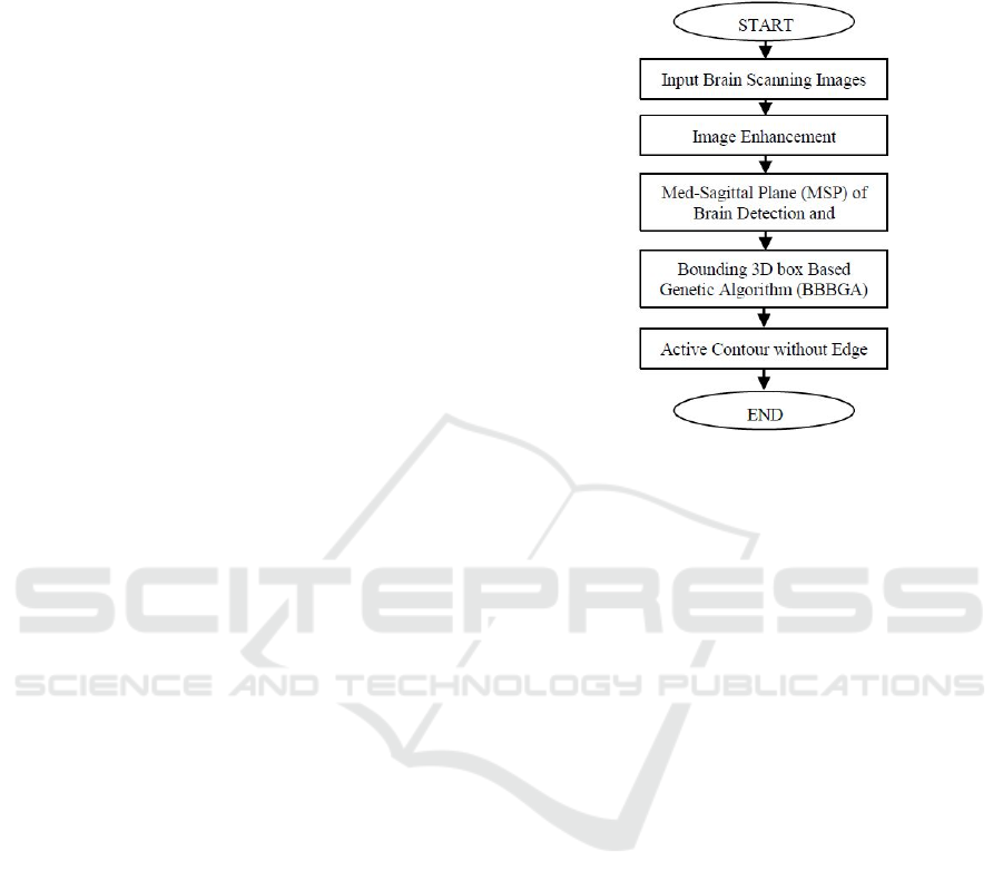
2 MATERIAL AND METHODS

The main objective of this research is to develop and

evaluate an automated algorithm for identifying the

location of tumours in MRI brain slices as well as

identifying the most important slices of pathological

patient to draw the attention of the clinicians to these

slices. The overall flow chart of the proposed

algorithm is shown in Fig. 1. It starts with the data

collection step from the Iraqi hospital, a set of

algorithms in the pre-processing stage and finally the

segmentation algorithm.

2.1 MRI Acquisition

Data collection is an important steps in this study. T2

and T1 weighted images of 88 pathological patients

were collected from the MRI Unit of Al Kadhimiya

Teaching Hospital in Iraq.

Each patient has 32 slices with a slice resolution

of (432×512 pixels), the inter-slice spacing is 5.5 mm,

and slice thickness is 5 mm. The MRI Unit in the

mentioned hospital has faced many problems in

diagnosing and issuing diagnostic reports for a large

number of inpatients and outpatients. The average

number of patients received daily by this unit is over

110 patients a days for a six working days week. Over

2400 patients are scanned monthly taking most of the

clinicians' time in diagnosing and interpreting MRI

slices. The dataset was collected using a SIEMENS

MAGNETOM Avanto 1.5 Tesla scanner. The

provided dataset consists of tumours with different

sizes, shapes, locations, orientations and types.

Figure 1: The Flow Chart of the proposed algorithm.

2.2 Image Pre-processing

Two preprocessing steps are performed on the MRI

brain scans; image enhancement and MRI intensity

normalization due to the intra-scan and inter-scan

image intensity variations and Mid-Sagittal Plane

detection and correction algorithm (Anju et al., 2013;

Lauwers et al., 2010; Aelterman et al., 2008; Bovik,

2009; Nabizadeh and Kubat, 2015).

2.2.1 Unifying the MRI Slices to 512×512

The provided MRI brain slices with a slice resolution

of (432×512) pixels and the proposed algorithm in

this study is implemented on squared slices of

(512×512) pixels. Therefore, the MRI slices are

resized by adding extra zeros' columns from left and

right till reaching to desired slice resolution.

2.2.2 MRI Image Enhancement

Image enhancement techniques are widely used to

refine medical images and improve the visibility of

the important structures in medical images. As well

as enabling the operators to see the details of the

medical image which may not be immediately

observable in the original medical image (Bankman,

2000; William, 2001). Generally, the spatial domain

techniques are more efficient computationally and

require less processing resources for implementation

(Gonzalez and Woods, 2002; Birry, 2013). The

BIOIMAGING 2016 - 3rd International Conference on Bioimaging

Gaussian filter is chosen for noise suppression in this

study due to its performance.

2.2.3 Mid-Sagittal Plane Detection and

Correction

The Mid-Sagittal Plane (MSP) identification is an

important step in brain image analysis as it provides

an initial estimation of the brain’s pathology

assessment and tumour detection (Jayasuriya and

Liew, 2012). The human brain is divided into two

hemispheres that have approximately a bilateral

symmetry around the MSP. This means that most of

the structures in one side of the brain have a

counterpart on the other side with a similar shape and

location. The two hemispheres are separated by the

longitudinal fissure that represents a membrane

between the left and right hemispheres (Ruppert et al.,

2011). The MSP extraction methods can be divided

into two groups (Ruppert et al., 2011; Liu, 2009);

Content-based methods that are based on finding a

plane that maximizes a symmetry measure between

both sides of the brain (Christensen et al., 2006;

Ardekani et al., 1997; Khotanlou et al., 2009; Ruppert

et al., 2011) and shaped-based methods that use the

inter-hemispheric fissure as a simple landmark to

extract and detect the MSP (Bergo et al., 2009; Liu,

2009).

In this study, we choose to determine the

orientation of the patient’s head instead of depending

on measuring the symmetry to identify the brain MSP

as we are using the principal components analysis

(PCA) method to compute the distinctive principle

axes that are orthogonal to each other. Those axes are

used to characterize the patient’s head by representing

the spatial distribution of the mass (Liu, 2009).

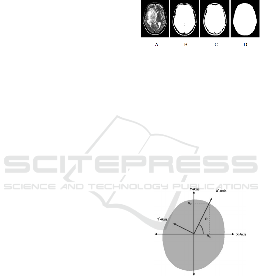
The proposed algorithm includes five steps; the

first step separates the brain from the background by

using the histogram thresholding approach because

the background normally has much higher number of

unavailing pixels (Nabizadeh, 2015).

The second step uses holes filling morphological

operator to fill the holes that are defined as a

background region of a binary image and surrounded

by connected borders of foreground (Dougherty,

2009; Bovik, 2009; Soille, 2003; Wilson and Ritter,

2000) as shown in Fig. 2.

The third step determines the orientation of the

patient's head using PCA. The PCA method

essentially attempts to transfer the coordinate of the

original data to a new coordinate system. Such that

the maximum variation in the data comes to lie on the

first coordinate. This is known as the first principal

component. The second maximum variation in the

data lies on the second coordinate and so on (Smith,

2002; Wallisch et al., 2014; Manly, 1988).

Figure 2: An example for MRI brain scanning image

segmentation, A) Original MRI image, B) Segmented MRI

image with threshold equal to 25, C) Dilated MRI image,

and D) Filled holes image.

The new coordinates of the given data are

estimated by calculating the eigenvectors which point

in the direction of the new dataset coordinates. The

desirable coordinate that has the highest eigenvalues,

passes through the maximum variation of data,

representing the orientation of the patient's head

(Wallisch et al., 2014). The angle θ between the X-

axis and X’-axis represents the degree of skewness of

the patient’s head during the MRI test as shown in

Fig. 3 and could be calculated using equation (1):

=tan







(1)

Where, V

and V

are the eigenvectors which are

related to the maximum eigenvalues.

Figure 3: Original and new coordinates of brain.

The fourth step is a Geometrical transformation

which is widely used in computer graphic and image

analysis. It is used to rotate and correct the patient's

head by the computedθ.

The fifth step is the positioning of the patient’s

head in the centre of the MRI image because

identifying the brain’s abnormality depends

essentially on measuring the symmetry between the

Automated Segmentation of Tumours in MRI Brain Scans

two brain’s hemispheres.

The MRI brain slices of each patient have the

same degree of skewness therefore the MSP detection

and correction algorithm is implemented on a single

slice instead of using all slices to avoid computational

complexity. The preferable slice for implementing the

MSP detection and correction algorithm is the slice

which is located in middle of the slices.

2.2.4 Exponential Transformation of MRI

Brain Slices

Exponential transformation is the process of

compressing the low contrast regions in an MRI brain

image and expanding the high contrast region in a

non-linear way. It is used to increase the intensity

difference between the brain tumour and the

surrounded soft tissue (Khandani et al., 2009). This

will help the GA to converge and move the generated

3D box faster and accurately to the abnormal region

of the brain.

3 BOUNDING 3D BOX BASED

GENETIC ALGORITHM

The novel BBBGA is proposed in this study to

identify the location of the tumours in MRI brain

slices automatically without the need for user

interaction. Where, a hundred of 3D boxes with

different sizes and locations are randomly generated

in the left hemisphere of the brain and these 3D boxes

are compared with the corresponding 3D boxes in the

right hemisphere of the brain through the objective

function. The 3D boxes are optimized and moved

using GAs towards the region that maximized the

objective function value. The objective function value

is high when the 3D boxes stands on the tumour

region and low when the 3D boxes stands on the soft

tissues because the tumour is always brighter than the

soft surrounding tissue of the brain (Khandani et al.,

2009). The output of BBBGA is the slices that contain

the tumour and corresponds to the optimized 3D box

that bounded the tumour over the relevant subset of

slices. The BBBGA method does not need image

registration nor intensity standardization in MRI

slices and is an unsupervised method.

3.1 The Design of the GA

There are several issues involved in designing GAs

such as individual size and population size in addition

to choosing the most appropriate operations such as

selection, crossover and mutation methods.

3.1.1 Individual Construction

As mentioned previously, the provided dataset of

MRI brain scanning slices were unified to (512 × 512)

pixels dimensions and each patient has 32 slices. The

3D boxes that are generated randomly in the left side

of the brain are compared with the corresponding 3D

boxes of the right side by using the fitness function.

The size of the search space will be (512 × 256 × 32)

pixels, and each generated 3D box is defined by six

variables that represent the coordinates of the 3D

boxes in the search space. Fig. 4 shows the original

generated 3D boxes by the GA, such that each

generated 3D box in the right hemisphere has a

corresponding 3D box in the right hemisphere.

Figure 4: Representation of one 3D box in the brain left

hemisphere using (x

, x

, y

, z

) coordinates and

opposite region.

Each individual in the GA population denotes the

binary representation of the coordinates of one 3D

box (x

, x

, y

, z

). Where, x

and x

represent

the height of the 3D box and are subjected to the

following constraints; 1≤ x

<512 and x

< x

≤512.

While y

and y

represent the width of the 3D box and

are subjected to the following constraints; 1≤ y

<256

and y

< y

≤256, and z

and z

represent the depth of

the 3D box and are subjected to the following

constraints; 1≤ z

<31 and z

< z

≤32. Fig. 5 shows

how the coordinates of the 3D box (x

, x

, y

, z

) are mapped to the individual of the GA in a binary

form where, this individual represents one 3D box

with the coordinates (135, 220, 23, 196, 10, 16).

Figure 5: Individual structure.

BIOIMAGING 2016 - 3rd International Conference on Bioimaging

and x

variables are composed of nine bits as

they vary from 1 to 512, while y

and y

variables are

composed of eight bits and vary from 1 to 256 and z

and z

variables are compose of five bits and vary

from 1 to 32. Subsequently, the individual size

becomes equal to 44 bits. By using the objective

function, we can measure the performance of

individuals in the problem domain (Chipperfield et

al., 1994). In this study, the fittest individuals that

have the highest numerical value of the associated

objective function are preserved. The objective

function g that is used in this study is based on finding

the absolute value of subtracting the means of the

intensities inside the generated 3D box in the left

hemisphere from the corresponding 3D box in the

right hemisphere using equation (2):

I



(i,j,k)−I



(i,j,k)

,,

,,

,,

,,



(2)

Where x, y and z are the coordinates of the generated

3D box on the left hemisphere and the corresponding

opposite region in the right hemisphere.

4 TUMOUR SEGMENTATION

USING 3D ACTIVE CONTOUR

WITHOUT THE EDGE

METHOD

The principle goal of the segmentation process is to

partition a medical image into sets of regions. It is an

important step in medical image processing and has

been used in many medical applications (Bankman,

2000). The Active Contour approach, also known as

the Snakes method is the most popular method and

was introduced by Kass et al., (1988). It is a very

successful approach for image segmentation. It

generates a snake or contour within an image domain.

The contour can be moved and directed under the

effect of internal forces within the same contour and

external forces from the image data (Xi-ping et al.,

2002). The location of the contour in the given image

is associated with the energy function E which is,

minimum when the contour reaches the object

boundary within the image. Through an iterative

process the contour deforms and the associated

energy is updated until reaching the minimum value

or the maximum number of iteration is reached. In

this study, we use the 3D active contour without edge

model as proposed by Chan and Vese (2001). This

model can detect object boundaries with or without

gradient, even when the object boundaries are very

smooth or with discontinuity because the main idea

of this method is to consider also the information

inside the object not only at its boundaries (Rousseau,

2009, Klotz, 2013). To fully segment the tumour, the

3D active contour without edge method is applied on

all MRI brain slices of each patient, where the initial

contour is defined as a 3-dimensional 3D box inside

the desired object and optimally selected by the

BBBGA method. The segmentation of all patients

were compared with the reference image (manual

segmentation) which is segmented by experts, such

that the true positive (TP) represents the number of

pixels which are correctly segmented, the false

positive (FP) represents the number of pixels which

are incorrectly segmented, the false negative (FN)

represents the number of pixels which are available in

the reference image and outside the segmented image

by the proposed algorithm, and the true negative (TN)

represents the summation of TP, FP and FN rates

(Anbeek et al., 2005). The accuracy of segmentation

is defined as follows (Nabizadeh and Kubat, 2015):



=

(+)

(+++)

×100

(3)

5 EXPERIMENTAL RESULTS

AND DISCUSSION

To evaluate the proposed algorithms which were

proposed in this study a set of examples will be

implemented using these algorithms.

5.1 MSP Detection and Correction

Results

Fig. 6 shows examples of detecting and correcting the

MSP of the brain of three MRI brain scanning images

which are oriented with different directions. The MRI

brain scanning image is shown in Fig. 7, is re-sampled

using the Geometric Rotator system object in

MATLAB Image Processing Toolkit (Matlab, 2013),

to rotate the patient’s head with different yaw angles

from -10 to 10 degrees in 5 degree intervals. The

proposed algorithm is evaluated by comparing the

achievable results with the proposed algorithms in

(Liu and Collins, 1996) as shown in Table 1. It is

noted that there is a significant difference in the mean

squared error (MSE) between the proposed

algorithms.

Automated Segmentation of Tumours in MRI Brain Scans

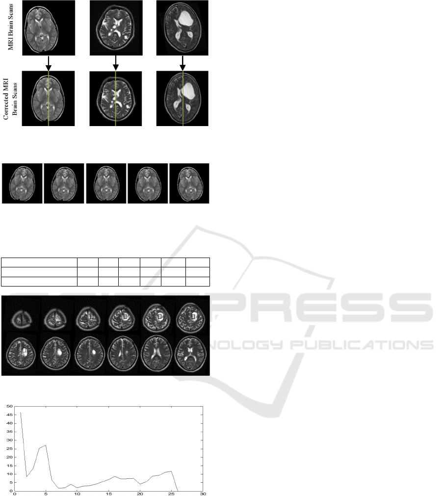
Figure 6: MSP detection and correction of three

pathological patients.

Figure 7: Re-sampling of one slice from the axial MRI brain

scanning image with varied rotate angles.

Table 1:

Numerical results of detecting yaw angle.

Yaw Angle -10 -5 0 5 10 MSE

Computed Yaw Angle -9.1 -4.7 0.5 5.4 10.5 0.3

(Liu and Collins, 1996) -8.5 -3 1.25 6.5 11.2 2.87

Figure 8: MRI brain scanning slices.

Figure 9: RMSE over 27 iterations by GA.

Once the patient's head is corrected, we apply the

BBBGA method to localize the brain tumour. Fig. 8

shows the output of BBBGA implementation on MRI

brain scanning slices of pathological patient with a

population size equal to 100 and a mutation rate equal

to 0.05. The optimal selected slices are 3 to 7. Fig. 9

shows how the RMSE decreases to the minimum

value within 27 iterations of GA. The achievable

accuracy by BBBGA was 95%, such that, there were

only 4 cases where the system has failed to identify

the abnormality because of the tumour's size is less

than 1 cm

5.2 Tumour Segmentation Results

Fig. 10 shows the result of segmentation of a

pathological patient, who has a brain tumour starting

from slice 2 and ending in slice 9. The MRI scans in

the dataset are manually segmented by expert and the

achievable segmentation accuracy was 90±3.7% by

3D Active Contour without Edge method. The same

dataset was segmented by 2D Active Contour without

Edge method and the achievable accuracy was

86.9±3.7%. Fig. 11 shows a comparison between the

3D and 2D segmentation of given dataset, such that it

is noted that the 3D segmentation outweighs the 2D

segmentation for all patients in the given dataset.

Subsequently, it is possible to identify the most

relevant slices to draw the attention of the clinicians

about these slices instead of spending long time on

diagnosing and interpreting MRI slices. Fig. 12 shows

a comparison of identifying clinically and

experimentally the most relevant slices for the

provided pathological patients after segmentation.

We have test the null hypothesis to prove that there is

no significant difference was found between

automatic and manual identification of slices showing

the tumor (t-test, p=0.86).

6 CONCLUSION

This paper presented an automated system that is able

to detect the location of tumour and then segment it

automatically in addition to identifying the most

relevant slices that should be diagnosed by clinicians

without requiring to inspect all patients’ slices.

The BBBGA method exploits the symmetry

feature of axial viewing of MRI brain slices to search

about the most dissymmetry region in the brain,

additionally it is unsupervised method meanwhile it

does need for training phase and it does not need for

image registration.

A major difficulty of segmentation with a white

matter tumours because of overlapping of the

intensity distributions of the white and grey matter.

As well as, some parts of the tumours in the grey

matter cannot be distinguished due to finite resolution

of the images and complicated shapes of the brain

tissues that impact on a large number of the voxels

which are located on the borders of tissues. In

addition, image intensity in the centre of tumour is

BIOIMAGING 2016 - 3rd International Conference on Bioimaging

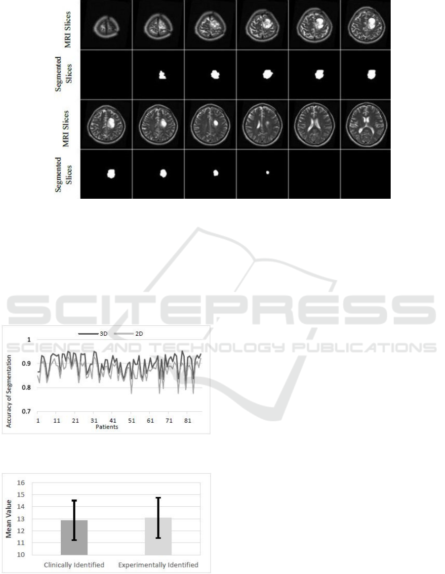
Figure 10: The result of segmentation of T2 weighted MRI brain slices by3D active contour without edge segmentation

method.

different from its Periphery. Therefore, the image

intensity at the borders of tumour may be the same as

grey matter. This phenomenon may cause confusion

between grey matter and tumours and result in

misclassification of the peripheral regions of the

tumours, which is occurred in T2 weighted.

Figure 11: Comparison between 3D and 2D segmentation

for given dataset.

Figure 12: Comparison between clinically and

experimentally MRI slice identification.

ACKNOWLEDGEMENTS

We would like to thank the MRI Unit in Al

Kadhimiya Teaching Hospital in Iraq for providing us

the diagnosed dataset of MRI brain scanning images.

REFERENCES

Aelterman, J., Goossens, B., Pizurica, A. & Philips, W.

2008. Removal of correlated rician noise in magnetic

resonance imaging. 16th European Signal Processing

Conference. Switzerland.

Anbeek, P., Vincken, L., Van Bochove, S., Van Osch, P. &

Van Der Grond, J. 2005. Probabilistic segmentation of

brain tissue in MR imaging. NeuroImage, 27, 795-804.

Anju, E., Karnan, M. & Sivakumar, R. 2013. MR brain

image classification with supervised bacteria foraging

technique using SVM. International Journal of

Futuristic Science Engineering and Technology, 1,

318-322.

Ardekani, A., Kershaw, J., Braun, M. & Kanno, I. 1997.

Automatic detection of the mid-sagittal plane in 3-D

brain images. IEEE Trans Med Imaging, 16, 947-52.

Bankman, I. (ed.) 2000. Handbook of medical imaging:

Academic Press, Inc.

Bauer, S., Nolte, L. & Reyes, M. 2011. Fully Automatic

Segmentation of Brain Tumor Images using Support

Vector Machine Classication in Combination with

hierarchical Conditional Random Field Regularization.

Medical Image Computing and Computer-Assisted

Intervention-Springer Berlin Heidelberg, 354-361.

Bergo, F., Falcão, A., Yasuda, C. & Ruppert, G. 2009. Fast,

Accurate and Precise Mid-Sagittal Plane Location in

Automated Segmentation of Tumours in MRI Brain Scans

3D MR Images of the Brain. Biomedical Engineering

Systems and Technologies. Springer Berlin Heidelberg.

Birry, R. 2013. Automated Classification in Digital Images

of Osteogenic differentiated stem Cells. PhD,

University of Salford, Manchester.

Bovik, A. 2009. The Essential Guide to Image Processing,

Elsevier Inc.

Chan, F. & Vese, A. 2001. Active contours without edges.

Image Processing, IEEE Transactions, 10, 266-277.

Chipperfield, A., Fleming, P., Pohlheim, H. & Fonseca, C.

1994. Genetic Algorithm TOOLBOX for Use with

MATLAB.

Christensen, J., Hutchins, G. & Mcdonald, C. 2006.

Computer automated detection of head orientation for

prevention of wrong-side treatment errors. AMIA Annu

Symp Proc, 136-40.

Dougherty, G. 2009. Digital Image Processing for Medical

Applications.

Gonzalez, R. & Woods, R. 2002. Digital Image Processing.

Jayasuriya, S. & Liew, A. 2012. Symmetry plane detection

in neuroimages based on intensity profile analysis.

Information Technology in Medicine and Education

(ITME), International Symposium on. Australia IEEE.

Kaal, E. C. & Vecht, C. J. 2004. The management of brain

edema in brain tumors. Current opinion in oncology,

16, 593-600.

Kass, M., Witkin, A. & Terzopoulos, D. 1988. Snake:

Active Contour Models. International Journal of

Computer Vision, 1, 321-331.

Khandani, M., Bajcsy, R. & Fallah, Y. 2009. Automated

Segmentation of Brain Tumors in MRI Using Force

Data Clustering Algorithm. Advances in Visual

Computing. Springer Berlin Heidelberg.

Khotanlou, H., Colliot, O., Atif, J. & Bloch, I. 2009. 3D

brain tumor segmentation in MRI using fuzzy

classification, symmetry analysis and spatially

constrained deformable models. Fuzzy Sets and

Systems, 160, 1457-1473.

Klotz, A. 2013. 2D and 3D multiphase active contours

without edges based algorithms for simultaneous

segmentation of retinal layers from OCT images. MS.c,

University of Texas at Austin.

Lauwers, L., Barbé, K., Van Moer, W. & Pintelon, R. 2010.

Analyzing Rice distributed functional magnetic

resonance imaging data: a Bayesian approach.

Measurement Science and Technology, 21, 115804.

Liu, S. 2009. Symmetry and asymmetry analysis and its

implications to computer-aided diagnosis: A review of

the literature. Journal of Biomedical Informatics, 42,

1056-1064.

Liu, Y. & Collins, R. 1996. Automatic Extraction of the

Central Symmetry (MidSagittal) Plane from

Neuroradiology Images. Robotics Institute, Carnegie

Mellon University.

Manly, B. 1988. Multivariate Statistical Methods A primer,

Department of mathematics and statistics, university of

Otago.

Matlab 2013. The Math Works kit.

Mikulka, J. & Gescheidtov, E. 2013. An Improved

Segmentation of Brain Tumor, Edema and Necrosis.

Progress In Electromagnetics Research Symposium

Proceedings, Taipei.

Nabizadeh, N. 2015. Automated Brain Lesion Detection

and Segmentation Using Magnetic Resonance Images.

PhD, University of Miami.

Nabizadeh, N. & Kubat, M. 2015. Brain tumors detection

and segmentation in MR images: Gabor wavelet vs.

statistical features. Computers & Electrical

Engineering.

Ray, N., Greiner, R. & Murtha, A. 2008. Using Symmetry

to Detect Abnormalies in Brain MRI. Computer Society

of India Communications, 31, 7-10.

Rousseau, O. 2009. Geometrical Modeling of the Heart.

Ph.D, University of Ottawa.

Ruppert, G., Teverovskiy, L., Chen-Ping, Y., Falcao, X. &

Yanxi, L. A new symmetry-based method for mid-

sagittal plane extraction in neuroimages. Biomedical

Imaging: From Nano to Macro, International

Symposium on, 2011 Chicago, IL. IEEE, 285-288.

Shen, S., Sandham, W., Granat, M. & Sterr, A. 2005. MRI

fuzzy segmentation of brain tissue using neighborhood

attraction with neural-network optimization.

Information Technology in Biomedicine, IEEE

Transactions on, 9, 459-467.

Smith, L. 2002. A tutorial on Principal Components

Analysis.

Soille, P. 2003. Morphological Image Analysis: Principles

and Applications, Springer-Verlag New York, Inc.

Wallisch, P., Lusignan, M., Benayoun, M., Baker, T.,

Dickey, A. & Hatsopoulos, N. 2014. Matlab for

Neuroscientists, Elsevier.

William, K. 2001. Digital Image Processing, Canada,

Wiley-Interscience.

Wilson, J. & Ritter, G. 2000. Handbook of Computer Vision

Algorithms in Image Algebra, CRC Press, Inc.

Xi-Ping, L., Jie, T. & Yao, L. 2002. An Algorithm for

Segmentation of Medical Image Series Based on Active

Contour Model. Journal of Software, 13, 1050-1058.

BIOIMAGING 2016 - 3rd International Conference on Bioimaging