Evaluation of Sharpness Measures and Proposal of a Stop Criterion for

Reverse Diffusion in the Context of Image Deblurring

Pol Moreno and Felipe Calderero

Department of Information and Communication Technology, Pompeu-Fabra University, Barcelona, Spain

Keywords:

Heat Equation, Reverse Diffusion, Sharpness Measures, Deblurring.

Abstract:

The heat equation can be used to model the diffusion process shown in a defocused (blurry) region of a picture

taken with conventional camera lens. The original focused image can be recovered by reverting the heat

equation, that is, by reverse diffusion. However, the main difﬁculty with this technique is that it becomes

unstable very quickly due to the ﬁnite precision of pixel values and the image values blow up. For that reason,

detecting the exact time when the reverse diffusion process should stop is crucial. The goal of this work it to

evaluate the behavior of different non-reference state-of-the-art sharpness measures (that is, when a perfectly

focused image is not available) for the forward and inverse diffusion processes and to propose a robust stop

criterion to reliably detect the moment before each region becomes unstable. To ﬁnd out a good stop criterion,

we carry out a set of experiments with test and real images. The results in this paper can be valuable not only

to estimate monocular depth from blur cues, but also to any other image processing ﬁelds that require image

deblurring.

1 INTRODUCTION

Retrieving the depth structure of a scene has been

an active research topic for many decades in com-

puter vision (Forsyth and Ponce, 2002). While most

approaches of depth estimation use multiple obser-

vations of a single scene (Rajagopalan et al., 2004),

(Favaro et al., 2008), not much has been proposed to

tackle the challenging task of retrieving the depth us-

ing a single observation taken with a camera with un-

known calibration. This general problem is known as

monocular depth estimation, and aims at recovering

relative depth information from a single image. Some

approaches have been proposed that exploit the occlu-

sion cues present on the image, for instance, learning-

based approaches (Hoiem et al., 2011), (Saxena et al.,

2008), and T-junction detection and interpretation ap-

proaches (Dimiccoli and Salembier, 2009), (Palou

and Salembier, 2011).

Other important cues, such as the blur effect

present in the objects further or closer than the depth-

of-ﬁeld of the camera, have received few attention in

the literature. To our knowledge, one of the most re-

cent works has been proposed by (Namboodiri and

Chaudhuri, 2008), where the heat equation is used

to model the image defocus process. The reverse of

the heat equation is applied to undo the blurring ef-

fect and the “time” it takes to recover each deblurred

region is proportional to its relative depth. This re-

verse diffusion process is ill-posed and becomes un-

stable very quickly. The authors use a threshold on the

mean of the gradient in a small neighborhood, but the

results provided by this approach are very noisy and

unstable. The consequence of the low quality of the

deblurring process forces to introduce a strong reg-

ularization based on Markov Random Fields that, in

turn, leads to highly smooth results and a poor resolu-

tion in terms of relative depth. This is just one exam-

ple of the impact that a robust strategy to detect when

the reverse diffusion process becomes unstable would

have in computer vision.

Motivated by the described monocular depth

framework, the goal of this work aims at studying

the sensitivity of a set of sharpness measures to detect

the moment where reverse diffusion becomes unsta-

ble, and to propose a robust stop criterion. Sharpness

measures can be classiﬁed in three categories: full-

referenced, reduced-referenced and non-referenced.

Full-referenced are a type of objective metric in which

a given image is compared to the original unaltered

version. In the reduced-referenced case, partial in-

formation of the original image is available and usu-

ally described by a set of local features. Neverthe-

less, image deblurring and monocular depth estima-

Moreno P. and Calderero F..

Evaluation of Sharpness Measures and Proposal of a Stop Criterion for Reverse Diffusion in the Context of Image Deblurring.

DOI: 10.5220/0004271200690077

In Proceedings of the International Conference on Computer Vision Theory and Applications (VISAPP-2013), pages 69-77

ISBN: 978-989-8565-47-1

 2013 SCITEPRESS (Science and Technology Publications, Lda.)

tion applications have no information about the con-

tent of the original (perfectly focused) image. For that

reason, in this work we have selected four state-of-

the-art non-referenced sharpness measures (Ferzli and

Karam, 2009) based on different features, such as im-

age statistics and frequency content. In this selection

we have considered those approaches that can be ap-

plied at a local spatial scale and, hence, can be consid-

ered as information measures in scale-space (Sporring

and Weickert, 1999), since our intention is not to eval-

uate the sharpness/quality of a whole image, but the

sharpness of an image region.

The organization of the rest of this paper fol-

lows. Section 2 presents the four state-of-the-art non-

reference sharpness metrics. In Section 3, we exper-

imentally study the behavior and sensitivity of each

measure to forward and reverse diffusion. A reduced

set of measures showing a good behavior are further

analyzed. Particularly in Section 3.1, for one of the

previous techniques we propose an strategy to detect

the time where the reverse diffusion should be stop

to prevent that the image blows up. Experiments on

real and test images are shown in Section 4. Finally,

conclusions are outlines in Section 5.

2 NON-REFERENCED LOCAL

SHARPNESS MEASURES

This section presents four non-referenced state-of-

the-art techniques that can be applied to measure the

local sharpness of an image region.

2.1 Variance

One of the simplest local sharpness measures is the

variance of an image window. That is,

var

) =

∑

(x,y)∈Ω

[u(x,y) −u]

(1)

where Ω

is a support window around pixel x

and N is the total number of pixels in the support win-

dow; u(x, y) is the image; and u is the mean value of

the image in the window. The variance is a very sim-

ple and efﬁcient metric that is quite robust to noise

and, intuitively, its value increases as the image gets

sharper since the intensity variation will be higher

than blurred images (Batten, 2000).

2.2 Sum of Modiﬁed Laplacians (SML)

Another family of metrics are based on the computa-

tion of second-order derivatives of the image, particu-

larly, the Laplacian. This type of metrics act as a high

pass ﬁlter in the frequency domain. Thus, they are

characterized by a good degree of accuracy but they

are very sensitive to noise (since they are based on

the direct computation of image derivatives). Partic-

ularly, here we analyze the Sum of Modiﬁed Lapla-

cians (SML), that is given by the following formula

(Aydin and Akgul, 2008):

SML

) =

∑

(x,y)∈Ω

ML(I(x, y)) (2)

where Ω

is a support window around pixel x

and ML(I(x,y)) is the modiﬁed Laplacian measure

given by:

ML(I(x, y)) = |−I(x + s, y) + 2I(x,y) −I(x −s, y)|

+ |−I(x, y + s) + 2I(x,y) −I(x, y −s)|

The reason to compute the absolute value of the

Laplacian is to avoid that the horizontal and verti-

cal derivatives may cancel each other. Here, s is

a step variable that is used to set the distance be-

tween the central pixel and the pixels used to com-

pute the second order derivative. Using different s

values may be useful to cope with different sizes of

texture elements. In our experiments, a value of s = 1

was found to produce the best results. The modiﬁed

Laplacian measure can be interpreted as an approxi-

mation of the Frobenius matrix norm (Horn and John-

son, 1990) of the Hessian matrix, which introduces

some connections with the detection of salient image

points provided by Lindeberg’s blob detector (Linde-

berg, 1993).

2.3 Frequency Metric

This image sharpness metric has been introduced by

(Shaked and Tastl, 2005). The sharpness is measured

by means of a localized frequency analysis. If u(x,y)

is an image, and |U(ξ

,ξ

)| is its magnitude spec-

trum, the fractal image model proposed in (Shaked

and Tastl, 2005) states that natural images follow a

fractal behavior given by

|U(ξ

,ξ

)| =

||(ξ

,ξ

)||

2H+2

(3)

where α is a constant, H is the Hurst parameter (Man-

delbrot and Wallis, 1969), and ||·||

refers to the Eu-

clidean norm.

According to this model, it is theoretically pos-

sible to reconstruct the original image if the Hurst

parameter H is known. While this is not realistic,

it comes to show that the frequency distribution can

certainly be useful to estimate an image degradation

(for instance, due to blurring). Finally. their proposed

VISAPP2013-InternationalConferenceonComputerVisionTheoryandApplications

measure is implemented by the ratio between the out-

put energy of a high pass ﬁlter and a band pass ﬁlter,

given by

f m

) =

∑

(x,y)∈

Ω



(x,y)



dx dy (4)

where

Ω

is the feature window around the pixel

determined by having the value of the band pass

ﬁlter larger than a threshold T:

Ω

= {(x,y) ∈

Ω

|BP

(x,y) > T } (5)

as suggested in (Shaked and Tastl, 2005), the value

of T was set to 50. HP

and BP

correspond to the

output of the high pass and band pass ﬁlters, respec-

tively:

(x,y) = (hp ∗m)(x,y) (6)

(x,y) = (bp ∗m)(x,y) (7)

where hp(x,y) and bp(x,y) are impulse responses of

high pass and band pass ﬁlters. However, for com-

putational efﬁciency they are implemented by inﬁnite

impulse response (IIR) ﬁlters, using recurrent ﬁnite-

differences input-output equations.

2.4 Thresholded Frequency Metric

A simpler frequency metric we have also studied is

based on computing the sum of all values of the im-

age spectrum in a certain range given by a frequency

threshold T (Batten, 2000), that is:

t f m

) =

∑

,ξ

∈[−T,T ]

|U(ξ

,ξ

)| (8)

where |U (ξ

,ξ

)| is the magnitude of the Fourier

transform of the subimage u(x,y). If T is too low,

some relevant frequency components can be missed

and the measure becomes less reliable. Following

(Batten, 2000), the value of T was set to 50.

2.5 Sharpness Index

The authors of (Blanchet et al., 2008) recently pro-

posed an image sharpness indicator based on the

Fourier phase spectrum (the argument of each Fourier

coefﬁcient), which contains crucial information about

the image geometry and, particularly, about its con-

tours. The main idea is that measuring the amount

of phase coherence in an image is related to measur-

ing the quality of the transitions between ﬂat regions

(that is, the edges). In other words, phase coherence

provides information about boundary alignment that,

in turn, is related to image sharpness. They deﬁne a

metric called Global Phase Coherence based on the

relative regularity (total variation) of images with all

possible phase functions. The periodic total variation

is given by:

TV (u(x)) =

∑

|x−y|=1

|u(x) −u(y)|, (9)

where u(x) is the image value at point x ∈ Ω ⊂ ℜ

and the difference x −y is modulo Ω. Here, it is as-

sumed that among all possible odd phase function ψ,

there will be some which will produce a more likely

image p(u

) > p(u). This comparison is equivalent to

comparing TV (u

) with TV (u). Finally, the Global

Phase Coherence is deﬁned as:

GPC(u) = −log



{ψ ∈ ρ, TV (u

) ≤ TV (u)}



|ρ|

where ρ is the vector space of all odd phase functions

and |S| denotes the Lebesgue measure (the length) of

a set S. In other words, it is a measure of the rela-

tive volume of phase functions that produce images

no less “plausible” than u.

Their proposed solution is to use a Monte-Carlo

simulation to impose random phases on u. This

approach is unfeasible for our purpose due to time

constraints. However, in a more recent publication

(Blanchet and Moisan, 2012), they propose an equiv-

alent sharpness measure, called Sharpness Index, that

can be computed much more efﬁciently. The key dif-

ference is that they consider Gaussian random ﬁelds

instead of random phase images. This allows replac-

ing the unfeasible probability by a Gaussian approx-

imation. This is done by estimating the probability

that a random image has a given total variation:

) = −log





µ −TV (u)



, (10)

where µ and σ are the expectation and standard devi-

ation of TV ( ˆu), respectively; ˆu = u∗w is the result of

convolving the original (sub)image u with a standard

white noise random image w, that is, an image with

all its values being independent random variables fol-

lowing a normal distribution. Finally, φ(x) is the tail

of the Gaussian distribution:

φ(x) =

√

2π

+∞

−t

Implementation details included transforming the

original image into a periodically smooth version,

(Moisan, 2011), to avoid border effects when com-

puting the periodic total variation and convolutions.

EvaluationofSharpnessMeasuresandProposalofaStopCriterionforReverseDiffusionintheContextofImage

Deblurring

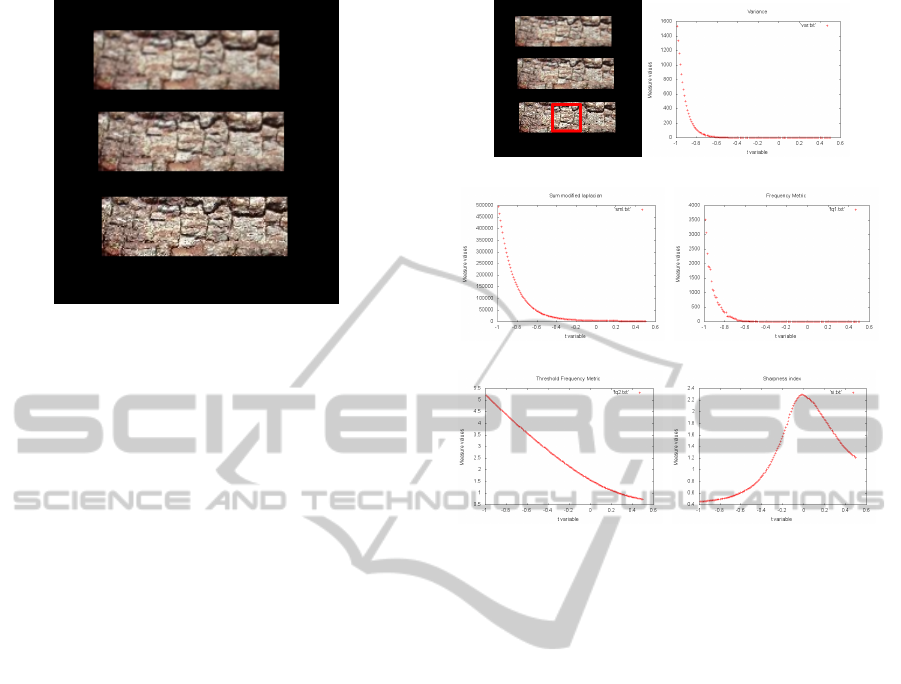
Figure 1: Synthetic image formed by a copy of a natural

texture with different degrees of blur. Bottom texture: orig-

inal (no blur). Middle texture: gaussian blur with 0.3 pixels

of standard deviation. Top texture: gaussian blur with 0.6

pixels of standard deviation.

3 SHARPNESS MEASURES

BEHAVIOR FOR REVERSE

DIFFUSION

The set of experiments in this section are designed to

test whether the sharpness measures presented in Sec-

tion 2 provide information about the reverse diffusion

process becoming unstable and, thus, they can be used

as stop criterion for image deblurring. For that pur-

pose, each experiment consists in analyzing the evo-

lution of the four sharpness measures of a region as

we forward or reverse the heat equation. We select a

synthetic image formed by a copy of a natural texture

with different degrees of blur (as explained in Figure

1, the bottom texture has no blur, the middle texture

has a Gaussian blur with a standard deviation of 0.3

pixels, and the top texture has a Gaussian blur with a

standard deviation of 0.6 pixels). From the top to the

bottom, the natural textures suffer from less blurring

(the bottom texture being perfectly focused).

First of all, we propose three different experi-

ments, where each experiment analyzes a window of

one of the natural textures (highlighted by a red box)

with different degrees of blur. In each experiment,

we ﬁrst apply the forward heat equation on the cor-

responding image region for a time interval of 0.5

time units (which means we are blurring it). Then,

we apply the reverse heat equation for a time inter-

val of 1.5 time units. Hence, we are covering a time

interval of [−1, 0.5] time units (notice that reversing

the heat equation means going backwards on our time

variable). This way, at time t = 0 we should get the

original image region. For the deblurred texture (bot-

(a) Region (b) Variance

(e) Threshold frequency (f) Sharpness index

Figure 2: Time evolution of the sharpness measures for a

region of the focused texture (marked by a red box in (a)).

tom of Figure 2(a)) the reverse diffusion should be

stopped around t = 0. For the other two textures on

top, the reverse diffusion should be stop at a negative

time (more negative for the upper texture), since those

image regions are blurred and need that the diffusion

process is reversed in order to recover a focused ver-

sion.

Figure 2 shows the time evolution of the four

sharpness measures for a region of the focused tex-

ture (red box in Figure 2(a)). Figure 3 outlines the

results for a region of the blurred texture in the mid-

dle (Figure 3(a)), and Figure 4 for a region of the top

and most blurred texture (Figure 4(a)).

The ﬁrst thing we notice is that the variance, the

Sum of Modiﬁed Laplacians, and the measures based

on the frequency domain all behave in a similar man-

ner: they increase monotonically as we deblur the im-

age (or in terms, of time units, they are monotonically

decreasing functions of time). Observing the three ex-

periments, the question we have to answer is how to

know when the reverse diffusion process should be

stopped. The variance for instance, while being very

computationally efﬁcient, offers very little insight on

the moment it becomes unstable (the steepness of the

curvature starts roughly at the same time on the three

experiments). The SML measure seems more sensi-

tive to the image changes as we deblur it. In particu-

VISAPP2013-InternationalConferenceonComputerVisionTheoryandApplications

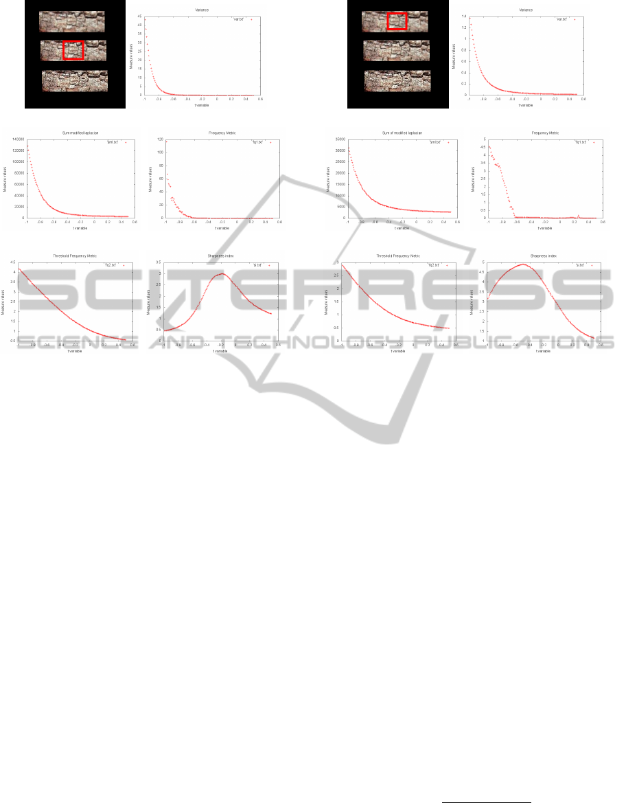
(a) Region (b) Variance

(e) Threshold frequency (f) Sharpness index

Figure 3: Time evolution of the sharpness measures for a

region of the mildly blurred texture (marked by a red box in

(a)).

lar, the sudden increase in the curvature of the graph

can be a good candidate for stop criterion. We ana-

lyze in more detail this option in Section 3.1.

The results for the ﬁrst frequency based measure

look too unreliable and there is no clear relation be-

tween the measure and the expected time to stop the

process. Finally, the frequency measure based on a

threshold behaves very similarly in the three tests,

which is a hint that it is not very useful for our pur-

pose.

In contrast to the previous measures, the Sharp-

ness Index shows a very interesting behavior. The ﬁrst

we notice is that it does not monotonically increase as

we sharpen the image region but, instead, it shows

a maximum at a certain time value. This may be a

consequence of being a more general quality measure

that takes into account not only blur, but also noise

and other degrading factors, and its peak provides the

time at which the image has the highest quality. If this

hypothesis is true, then comparing the time at which

this measure peaks should provide information about

the degree of defocus that should be applied to a cer-

tain region. Indeed, for the experiment with the region

in the focused region (Figure 2), the peak is very close

to t = 0; for the experiment with the semi-blurred tex-

ture (Figure 3), the measure peaks closer to t = −0.2;

and for the last experiment, the most blurred region in

(a) Region (b) Variance

(e) Threshold frequency (f) Sharpness index

Figure 4: Time evolution of the sharpness measures for a

region of the highly blurred texture (marked by a red box in

(a)).

Figure 4, the peak is located at roughly t = −0.5. This

in fact gives us a correct estimation of the amount of

blur of each one of the regions.

So far, the Sharpness Index seems to be the most

interesting measure, but due to the complexity of the

measure, we would like to explore also the use as a

much more simple measure as the Sum of the Modi-

ﬁed Laplacian (SML). Nevertheless, since the SML is

monotically decreasing with the degree of blur and,

hence, it does not present a maximum for the stop

time as the Sharpness Index, we propose to analyze

the evolution of its curvature in order to see if a clear

stop criterion can be formulated. This is the goal of

the next section.

3.1 Maximum Curvature of the SML

The idea is to study the curvature of the SML and see

if there is a clear relation with the time the reverse

diffusion should stop and, for instance, the maximum

of the curvature. Recall that the signed curvature κ is

given by:

κ(t) =

SML

(t)

(1 + f

SML

(t))

3/2

(11)

where f

SML

is the second derivative of f

SML

computed

by ﬁnite differences:

EvaluationofSharpnessMeasuresandProposalofaStopCriterionforReverseDiffusionintheContextofImage

Deblurring

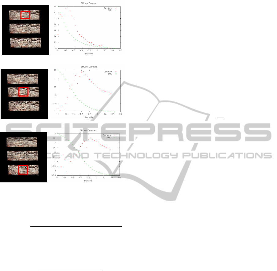
(a) Highly blurred (b) SML max. curvature

(e) Focused (f) SML max. curvature

Figure 5: Evolution of the SML and its curvature for the

regions with different degrees of blur shown in Figures 2, 3,

and 4, respectively from top to bottom.

SML

(x) =

SML

(x + c) −2 f

SML

(x) + f

SML

(x −c)

(12)

where c is the interval constant used in the heat equa-

tion, and f

SML

is given by

SML

(x) =

SML

(x + c) − f

SML

(x −c)

(13)

The time evolution of the curvature for each one

of the previous three experiments is shown in Figure

5. It can be seen that the time at which there is a

maximum curvature is an good indicator of when the

reverse diffusion is becoming unstable, similar to the

peak provided by the Sharpness Index but being much

simpler to compute. The deblurred images by inverse

diffusion according to the estimated blur value pro-

vided by the Sharpness Index and the SML maximum

curvature are shown in Figure 6.

To conclude, the Section 4 compares the perfor-

mance as stop criterion of both strategies: the maxi-

mum of the Sharpness Index and the maximum cur-

vature of the SML.

4 EXPERIMENTAL

COMPARISON

After analyzing the four state-of-the-art sharpness

measures in a set of test experiments in Section 3, we

have concluded that the two best strategies to be used

as stop criterion for reverse diffusion are the maxi-

mum of the Sharpness Index and the maximum cur-

vature point of the SML. We compare these two ap-

proaches with the stop criterion used in (Namboodiri

and Chaudhuri, 2008), in the context of recovering

relative depth from blur information in a single im-

age without knowing the camera parameters. This is

a very simple method based on computing the differ-

ence between the gradient at a pixel with the average

gradient of its neighborhood. This difference is com-

pared with a threshold |∇u −∇u| < Θ (where Θ is

between 0.2 and 0.4 in their experiments). The ex-

perimental results from their measure show that it is

not robust enough, and a spatial regularization by a

Markov Random Field approach over the local esti-

mation values is required.

In the recovery of relative depth information from

blur in a single image, we carry out an experiment on

the same synthetic image of three textures shown in

the previous section. This time, we divide the image

in squared regions of 15 ×15 pixels, and apply the

reverse heat equation algorithm for each region until

the stop criterion is reached. The time until the re-

verse diffusion process is stopped is proportional to

the relative depth of the corresponding region. Figure

7 shows the results for each one of the stop criteria

considered. The time values are normalized to the in-

terval [0, 1], and the darker a pixel, the closer it is to

the observer (less relative depth), and viceversa.

We can observe in Figure 7 how the three ap-

proaches work relatively well but also present some

inaccuracies. As we expected, the technique based on

the gradient stop criterion proposed in (Namboodiri

and Chaudhuri, 2008) shows quite an irregular depth

estimation on a small scale. Note that we are not test-

ing the full algorithm with the post-processing reg-

ularization they propose, but only the part up to the

stop criterion. However, we believe that an improve-

ment in the local depth estimation will simplify the

spatial regularization that the authors have to carry in

order to regularize the results or, even, will make it

not necessary.

The results for the depth estimation using the

Sharpness Index as stop criterion seem smoother than

the ﬁrst method but it still shows inaccurate depth val-

ues. While it is a promising feature due to the fact that

it actually measures a global image quality/coherence,

it still does not justify the high computational cost (it

VISAPP2013-InternationalConferenceonComputerVisionTheoryandApplications

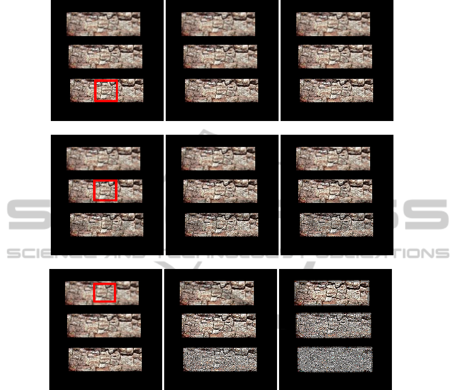
(a) Region (b) Sharpness Index (c) SML max. curvature

(d) Region (e) Sharpness Index (f) SML max. curvature

(g) Region (h) Sharpness Index (i) SML max. curvature

Figure 6: For each row, deblurred image according to the blur value estimated in a squared window of the original image

(ﬁrst column, red box) using the Sharpness Index (second row) and the SML maximum curvature (third row). Respectively

for the ﬁrst, second and third rows, the estimated blur is 0.0, 0.2, and 0.5 for the Sharpness Index; and 0.1, 0.3, 0.8 for the

SML maximum curvature.

took around 5 minutes to complete the depth estima-

tion, in contrast to the less than a minute time required

by the rest of the methods, using a 2.4 Ghz Intel Core

i5 desktop processor).

Lastly, our proposed technique seems to work bet-

ter than the other two in this synthetic image. The es-

timate is signiﬁcantly more regular along the surface

of each texture. As previously commented, this type

of result would make not necessary any further regu-

larization step for the relative depth estimation.

For the depth estimation around the edges, the

ﬁrst technique actually behaves quite well, with the

background-foreground separation we would expect.

However, for the other two techniques that is not the

case (the depth map surface is “larger” than the origi-

nal surfaces).

Another experiment in shown in Figure 8 for a nat-

ural image. We can observe that the Sharpness In-

dex is indeed not robust enough especially when it

comes to natural images in which the defocus effects

are much more unpredictable. Our intuition is that as

it is a statistical measure of the phase coherence, it is

a more useful technique to evaluate the whole image

sharpness than to evaluate small image regions, where

the statistical estimation it requires become much less

reliable.

The maximum curvature point of the SML pro-

vides the best results for this example and seems the

best candidate in terms of results and efﬁciency. In

addition it does not require to set any parameter or

EvaluationofSharpnessMeasuresandProposalofaStopCriterionforReverseDiffusionintheContextofImage

Deblurring

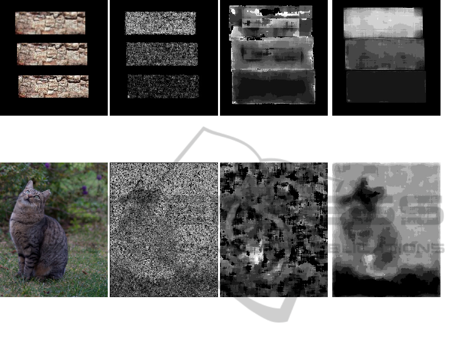
(a) Original image (b) (Namboodiri and Chaudhuri, 2008) (c) Sharpness index (d) SML max. curvature

Figure 7: Depth estimation of three textures with different stop criteria. The time values are normalized to the interval [0,1],

and the darker a pixel, the closer it is to the observer (less relative depth), and viceversa.

(a) Original image (b) (Namboodiri and Chaudhuri, 2008) (c) Sharpness index (d) SML max. curvature

Figure 8: Relative depth estimation for a single natural picture based on the time of reverse diffusion before unstability.

threshold as opposed to the gradient method in (Nam-

boodiri and Chaudhuri, 2008) .

5 CONCLUSIONS

Since the reverse heat equation is very ill-posed, it can

only be applied up to a certain point before it becomes

unstable. Therefore it is necessary to have a reliable

measure to detect this moment in order to achieve the

best results in image processing and computer vision

tasks requiring image deblurring.

In this work, we have evaluated a set of state-of-

the-art sharpness measures. We have also proposed

a method to extract information to stop the reverse

diffusion process for one of the techniques, particu-

larly, the Sum of the Modiﬁed Laplacians, based on

the maximum of its curvature.

In the context of image deblurring applied to re-

covering relative depth information from blur in a sin-

gle image, the proposed approach provides accurate

results with a reduced computational cost. Our cur-

rent work aims at providing further evaluation of this

measure in terms of size and shape of the image win-

dow used in its estimation, and applying it to solve

other image processing problems related to image de-

blurring and deconvolution.

REFERENCES

Aydin, T. and Akgul, Y. (2008). A new adaptive focus

measure for shape from focus. In Proceedings of the

British Machine Vision Conference, pages 8.1–8.10.

Batten, C. (2000). Autofocusing and astigmatism correc-

tion in the scanning electron microscope. PhD thesis,

University of Cambridge.

Blanchet, G. and Moisan, L. (2012). An explicit sharpness

index related to global phase coherence. In Acoustics,

Speech and Signal Processing (ICASSP), 2012 IEEE

International Conference on, pages 1065 –1068.

Blanchet, G., Moisan, L., and Roug

e, B. (2008). Measur-

ing the global phase coherence of an image. In Image

Processing, 2008. ICIP 2008. 15th IEEE International

Conference on, pages 1176–1179. IEEE.

Dimiccoli, M. and Salembier, P. (2009). Exploiting t-

junctions for depth segregation in single images.

In Acoustics, Speech and Signal Processing, 2009.

ICASSP 2009. IEEE International Conference on,

pages 1229–1232. IEEE.

VISAPP2013-InternationalConferenceonComputerVisionTheoryandApplications

Favaro, P., Soatto, S., Burger, M., and Osher, S. (2008).

Shape from defocus via diffusion. Pattern Analy-

sis and Machine Intelligence, IEEE Transactions on,

30(3):518 –531.

Ferzli, R. and Karam, L. (2009). A no-reference objective

image sharpness metric based on the notion of just no-

ticeable blur (jnb). Image Processing, IEEE Transac-

tions on, 18(4):717–728.

Forsyth, D. and Ponce, J. (2002). Computer vision: a mod-

ern approach. Prentice Hall Professional Technical

Reference.

Hoiem, D., Efros, A., and Hebert, M. (2011). Recovering

occlusion boundaries from an image. International

Journal of Computer Vision, 91(3):328–346.

Horn, R. and Johnson, C. (1990). Matrix analysis. Cam-

bridge university press.

Lindeberg, T. (1993). Detecting salient blob-like image

structures and their scales with a scale-space primal

sketch: a method for focus-of-attention. International

Journal of Computer Vision, 11(3):283–318.

Mandelbrot, B. and Wallis, J. (1969). Some long-run prop-

erties of geophysical records. Water resources re-

search, 5(2):321–340.

Moisan, L. (2011). Periodic plus smooth image decompo-

sition. Journal of Mathematical Imaging and Vision,

39(2):161–179.

Namboodiri, V. and Chaudhuri, S. (2008). Recovery of rel-

ative depth from a single observation using an uncali-

brated (real-aperture) camera. In Computer Vision and

Pattern Recognition, 2008. CVPR 2008. IEEE Confer-

ence on, pages 1–6. IEEE.

Palou, G. and Salembier, P. (2011). Occlusion-based depth

ordering on monocular images with binary partition

tree. In Acoustics, Speech and Signal Processing

(ICASSP), 2011 IEEE International Conference on,

pages 1093–1096. IEEE.

Rajagopalan, A., Chaudhuri, S., and Mudenagudi, U.

(2004). Depth estimation and image restoration using

defocused stereo pairs. Pattern Analysis and Machine

Intelligence, IEEE Transactions on, 26(11):1521 –

1525.

Saxena, A., Chung, S., and Ng, A. (2008). 3-d depth re-

construction from a single still image. International

Journal of Computer Vision, 76(1):53–69.

Shaked, D. and Tastl, I. (2005). Sharpness measure: To-

wards automatic image enhancement. In Image Pro-

cessing, 2005. ICIP 2005. IEEE International Confer-

ence on, volume 1, pages I–937. IEEE.

Sporring, J. and Weickert, J. (1999). Information measures

in scale-spaces. Information Theory, IEEE Transac-

tions on, 45(3):1051 –1058.

EvaluationofSharpnessMeasuresandProposalofaStopCriterionforReverseDiffusionintheContextofImage

Deblurring