
Effective Residual and Regional Gravity Anomaly Separation
Using 1-D & 2-D Stationary Wavelet Transform
Naeim Mousavi
1
, Vahid E. Ardestani
2
and Hassan Moosavi
3
1
Young Researchers Club & Elites, Hamedan Branch, Islamic Azad University, Hamedan, Iran
2
Institute of Geophysics, University of Tehran, Tehran, Iran
3
Rah Avard Danesh Institute Affiliated with Ministry of Training and Education of Iran, Hamedan, Iran
Keywords: Separation, Stationary Wavelet Transform, Gravity Data, Correlation Coefficient.
Abstract: Numerous studies on capabilities of de-noising and separation by wavelet were performed, and their all
aims more and less was elimination of possible largest nongeological factors, noise, and to achieve pure
regional effects free from residuals. De-noising could be used for removal of non-desired effects like
latitude, terrain, tides, drift etc., from our desired portion of data as target. Separations of anomalies that are
not of interest conclude shallow structure is suitable to be optimal. Hence detection and removal of ever
larger surface anomalies to obtain optimal separation is of interest. At up to now studies, large deviation of
primarily original signal has been prevented. In this paper controlling factors which limit the overall
deviation of transformed signal from the original one have been replaced with two new parameters that
simultaneously cause extracting the maximum surplus signals, residuals, and also preserving the original
form ever possible. Results of artificial models along with application of separation to real data indicate the
usefulness of discrete stationary wavelet transform in order to optimal separation of anomalies with various
wavelengths.
1 INTRODUCTION
The traditional Fourier-based low or high pass
filters, such as Butterworth and Wiener, attenuate
the effect of noise in the data, but these have a
severe effect on smoothing out high frequency
signals and do not always work well because
globally remove high frequencies. General
smoothing substantially broadens features of
interest while gravity data is globally smooth.
Moreover many geophysical signals are non-
stationary in nature, therefore analyzing either in
uniquely time or only frequency domain is not
appropriate since the main draw back of Fourier
domain processing is edge effect and global
denoising (Fedi et al, 2004).
The other conventional approach to high
frequency separation is to apply a Naudy style and
nonlinear statistical filter. Success of these methods,
is due to some prior knowledge of nature of the high
frequency components. The shortcomings of
Fourier and Nonlinear filtering are apparent and
pose limitations on the detail and accuracy of
information accessible (Leblanc and Morris, 2001).
As an innovative technology developing from the
1980’s, wavelet transform has been widely used in
geophysics for its characteristics such as time
frequency analysis, multi-resolution and
decorrelation (Yan and Wu, 2011).
Since wavelets can successfully decompose and
separate the signal into discrete levels, the
application of separation procedures can be
discriminately applied to these wavelet levels
(Leblanc and Morris, 2001). The result is to
effectively removal the contribution of the high
frequency component to the whole of the data, while
keeping the geologically significant data as free as
possible from the effects of the thresholding process.
The procedure to manipulate the coefficients to
force some parts to remain at or converge to a
specified value is known as thresholding.
Separation and denoising can be viewed as a very
practical and advanced form of thresholding.
Denoising of data sets using wavelet transform has
been performed by a number of researchers
(Donoho, 1993); (Donoho and Johnstone, 1994);
(Saito, 1994); (Coifman and Donoho, 1995);
(Moreau et al., 1999); (Ridsdill-mith and Dentith,
659
Mousavi N., E. Ardestani V. and Moosavi H..
Effective Residual and Regional Gravity Anomaly Separation - Using 1-D & 2-D Stationary Wavelet Transform.
DOI: 10.5220/0004219806590668
In Proceedings of the 2nd International Conference on Pattern Recognition Applications and Methods (PRG-2013), pages 659-668
ISBN: 978-989-8565-41-9
Copyright
c
2013 SCITEPRESS (Science and Technology Publications, Lda.)

1999). Soft thresholding has been applied to all the
data of this study. We consider the issue of high-
frequency components created by shallow micro-
anomalies and separation of them within the wavelet
transform domain. The minimum-risk method
simply minimizes a least-squares estimate of the
error involved in the difference between the true
reading and the best estimate of that reading. The
best estimate for the ideal threshold estimator using
soft thresholding is based on the standard deviation
of the high frequency components and the number of
sample points (Leblanc and Morris, 2001).
The
investigation by Neumann and von Sachs (1995) has
furthered the basis for the risk estimator to include
non-Gaussian distributions.
However, the micro-
anomalies (high frequency components) were
comprised of features that are of considerably
shorter wavelength than the portions of interest of
the signal.
The wavelet approach has minimized the
presence of the spikes without introducing the
effects of splining the signal that is seperated by the
wavelet process. In Lebelance study in 2001, the
nongeological components at times, are similar in
amplitude and wavelength to the signal of interest
therefore are considerably more difficult to
eliminate.
The intent of this work is to show the effects of
wavelet method on the removal of the largest
spikelike or high frequency features led to the
optimal (maximall) separation. Various of such
features, high frequency one, are including
measurement resulting from the imperfect
instruments, persoal error and superimposing by the
surface micro-anomalies which produce useless
high-frequency signals. Separation is denoted often
for residual distincting from regional that is
established in this study.
Such as these methods are
independent and have recognizable process for
separation.
2 WAVELET ANALYSIS
One of the most important characteristics of wavelet
transform is that continuous wavelet transforms have
an adaptive window in time-frequency space (Yan
and Wu, 2011), which is sharpened automatically
with high center frequency while broadened with
low center frequency. Thus, wavelet transforms can
offer high resolution for high frequency signals and
give information for low frequency signals
completely.
Wavelet coefficients are separated into different
scales corresponding to different degrees of
approximation to the original data. The lower
frequencies are represented by a small number of
large coefficients, mainly located at the coarse
scales, while high-frequencies are represented by a
large number of small coefficients at the finer scales.
Wavelet threshold separation is simply to keep
coefficients whose amplitudes are greater than a
specified threshold and discard the coefficients
smaller than the threshold (Yan and Wu, 2011).
Wavelet transform is applied as continuous and
discrete form. The overall effect of applying the
CWT is that it takes the wavelet function and
continuously dilates and translates it over the series.
2.1 Continous Wavelet
Continuous wavelet transform function
can be
expressed as follows:
,
,
,
,
(1)
The basis functions are defined as:
,
1
√
∗
,,∈,0
(2)
where a is the dilation parameter, b is the translation
parameter, and R is the set of all real numbers.
Multiplier
√
is used to normalize energy function
in different scales. Transform in wavelet domain is a
function of time and frequency simultaneously.
2.2 Discrete Wavelet
The CWT allows a fine decomposition of the space-
scale plane, but the dilated and translated versions of
the mother wavelet do not have orthogonal
properties. This property may be important, as in the
case of filtering with respect to position and scale
parameters, it can be useful to resort to orthogonal
bases discrete families of orthonormal wavelets.
Discrete families of orthonormal wavelets are
introduced as follows:
,
1
√
2
2
2
1
√
2
2
(3)
which are obtained by dilating or contracting and
translating ψ
0,0
, with the choice a = 2l and b = ka
with l, k
∈
Z (Z is the set of integers). In this case,
the discrete wavelet transform (DWT) is:
,
,
(4)
ICPRAM2013-InternationalConferenceonPatternRecognitionApplicationsandMethods
660

and the inverse discrete wavelet transform (IDWT)
is:
,
,
(5)
The discrete wavelet transform (DWT), using the
property of localization of wavelet bases has been
used as a powerful tool in filtering and separation
problems. The continuous wavelet transform (CWT)
exploits the upward continuation properties of the
field horizontal derivative and allows the location of
potential field singularities in a simple geometrical
manner (Fedi et al., 2004).
2.3 Thresholding
Separation is how to manipulate the wavelet
correlation coefficients produced by the DWT in
order to obtain the best residual-free data set, known
as smoothed out regional. Residuals in real data are
often seen as high-frequency or spike-like
components and predefined feature corresponds to
i.e. shallow micro-anomalies. With real data, there
are only two practical choices of thresholding: hard
or soft. With hard thresholding, all values of the
wavelet correlation coefficients below (or above,
depending on the application) the threshold value λ
are set to zero. In soft thresholding, the values
approach zero at a linear rate (Fedi et al., 2004).
The explicit difference between hard and soft
thresholding is when |x(t)| > λ. In the case |x(t)| ≤ λ,
λ for both hard and soft thresholding is zero. For
hard thresholding, λ is equal to x(t) but for soft
thresholding is determined by this equation:
sign(x(t))(|x(t)| − λ). Where x(t) is the value of the
wavelet correlation coefficient at some level
dependent observation points (Strang and Nguyen,
1996). Soft thresholding of these same data was
found to reconstruct the signal in a more continuous
form that did not induce obvious artefacts. This
same conclusion has been reached by other studies
(Donoho and Johnstone, 1994); (Moreau et al.,
1999) therefore, soft thresholding has been applied
to all the data of this study
3 GRAVITY DATA SEPARATION
TECHNIQUE
High frequency events are a drastic deviation from
the general trend of the local data in either frequency
content or amplitude or both (Fedi et al., 2000). In
the other words high frequency components is a
subjective feature of all real data. The perception of
what residual is and what it is not varies with the
intent of the end use of the data what may be
considered residual to one observer may be regional
to another. This leads to the realization that no
matter what the application is, a measured value will
always have some amount of unwanted signal. As a
result, the need for separating the unwanted portion
from the portion of interest is essential to all users
and is the motivational concept behind separation
(Leblanc and Morris, 2001).
Although separation methods have sound basis
for specific applications under specific conditions,
each has variable degrees of success when applied to
high frequency features such as aeromagnetic spike
anomalies. A data spike is a single point anomaly
whose magnitude is usually, but not necessarily, of
significant deviation from the trend of the data. It is
generally smaller in spatial extent and larger in
amplitude than the local trend of the geologically
sourced data. The ambiguity of this definition is a
result of the signal associated with non geologic
sources that cause the spike-like anomalies. These
sources include acquisition errors, levelling, latitude,
terrain, tides, drift etc. and shallow small anomalies.
Surface micro-anomalies create high-frequency
portion at signal. Sometimes the purpose of the
analysis is diagnosis of these shallow anomalies. In
such a case low pass filter damage useful
information of the data. Remember that random high
frequency signals can not always describe the
behaviour of gravity residuals; so the arithmetic is
used to remove such high frequency features have
limited application in practice.
Maximum (abs( main signal-long wavelength
signal produced by SWT))= Maximum Residual
(MR)
By applying the discrete stationary wavelet filter and
soft thresholding all high frequency effects are
removed. So, regression of the effects of surface
anomalies should be maximal. Continuity of soft
thresholding reduces the high frequency content of
signal that is occurred by growing scales until the
overall form of the signal has not been deformed.
An optimal separation also let the effect of
deeper anomalies that were not seen because of
micro anomaly is now evident. Minimum deviation
of processed signal under wavelet thresholding
occurs at lower scales. Going to larger scales causes
separation of larger residuals. The signal to noise
ratio or Regional to Residual Ratio (RRR) also
decreases with increasing scale. Since the residual
amplitude is in the denominator of the ratio, small
EffectiveResidualandRegionalGravityAnomalySeparation-Using1-D&2-DStationaryWaveletTransform
661
RRR is equivalent to large residual separation.
The shrinking process of the RRR continues until
that all the original signal is remarked as residual.
We seek smallest RRR until the amplitude of
transformed signal (regional signal) are not less than
one of detected signal as residual it means the best
case is that RRR is unit or one.
4 SYNTHETIC GRAVITY DATA
4.1 Maximum Residual Separation at
Minimum RRR
The simplest way to figure out the main concept of
residual at gravity data is to consider a shallow
smaller anomaly located over the bigger buried
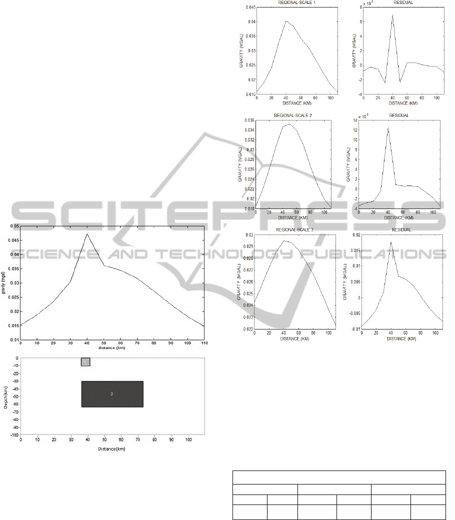
source (Fig.1).
Figure 1: synthetic model composed of two prisms. Prism
No.1 is nearer to the surface and smaller at size rather than
the other.
Both No.1 and No.2 prisms have the density
contrast of 0.1g/cm
3
. Shallow anomaly causes spike-
like effect at trace of deep structure and is
recognized as residual in this example. Residual
levels will not change much with the basic functions
and more is the function of scale selection (compare
results of Table 1 and 2).
We use Haar function at different scales to
decide about the level in which the best separation
result (unit or almost near unit RRR) is achieved.
a
b
c
Figure 2: separation of synthetic data steps by wavelet
transform. Three steps are due to scale 1, 2 and 3 are as
shown in part a, b and c. a) Application of wavelet at scale
1 with Haar basis function. b) Result of wavelet at scale 2
with Haar basis function. c) Regional and residual signal
reconstruction by wavelet at scale 3 with Haar basis
function. At three above sections the separated residual
signal, is shown at beside subplot.
Table 1: Maximum residual and regional to residual ratio
provided at different scales for synthetic data (Fig. 1).
Haar wavelet basis
Scale 1 Scale 2 Scale 3
MR RRR MR RRR MR RRR
0.006 2.597 0.012 1.058* 0.017 0.2991
The advantage of Haar function is exactly to
detect two distinct wave number levels that
accidentally this condition was occurred in this
synthetic. It does not mean that we have reached a
certain pattern and use only the Haar functions for
always separation process.
The lowest regional to residual ratio, also not
less than unit, is correspondent to the wavelet at
ICPRAM2013-InternationalConferenceonPatternRecognitionApplicationsandMethods
662
scale 2 (Table 1). Among all functions, Haar
produces the minimum acceptable RRR (Table 2).
As shown at Fig. 2(b) high-frequency effect of prism
No.1 is completely separated and regional signal
contains only the expectable anomaly.
Table 2: regional to residual ratio for different wavelet
functions at scale 2 for synthetic including two prisms.
Wavelet basis functions RRR
Haar 1.058732010890705*
dmey 1.863303773918932
Db1 1.058732010890705
Db2 1.453860116416355
Db3 1.615515002033936
Db4 1.710706620370309
Db5 1.772346126748260
Db6 1.814108360446961
Db7 1.835009919059236
Db8 1.843231484570417
Sym1 1.058732010890705
Sym2 1.453860116416355
Sym3 1.615515002033936
Sym4 1.710706620379929
Sym5 1.772346126737329
Sym6 1.814108360446384
Sym7 1.835009919053853
Sym8 1.843231484558451
Coif1 1.468967960816310
Coif2 1.727258582982356
Coif3 1.826747213107115
Coif4 1.846624829191316
Coif5 1.855111352245451
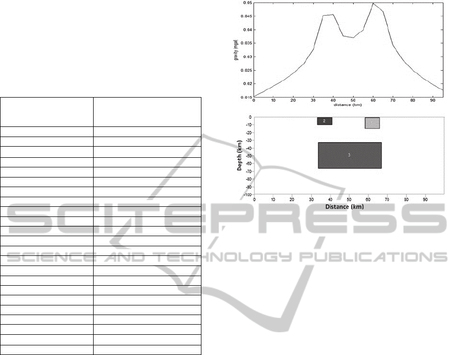
4.2 Maximized Separation by
Correlation Test
All three prisms at Fig. 3 have a density contrast of
0.1 g/cm
3
related to zero density of their
surroundings. Shallow prisms can be seen as the
agents that produce high frequency effects. Since
prism No. 2 is larger at size, has created signal with
bigger amplitude. Hence we expect that its trace is
completely clarified purely at the higher scales of
wavelet transform in which there is no effect of
prism No.2 surly.
Maximum residuals, regional to residual ratios
and correlation coefficients of wavelet at four scales
are given in Table 3. RRR at scale 3 is
approximately unit and the smallest one is obtained
again by Haar function at this scale like previous
synthetic. The separation procedure is led to signal
completely deformation when using wavelets at
scale rather than 3. In this level whole change in
signal shape is so much large that is not entitled
residual of data by SWT likewise is more similar to
original signal.
Figure 3: Synthetic model composed of three prisms.
Prisms No.1 and No.2 are nearer the surface and smaller at
size rather than No.3. Two spike-like anomalies created by
shallow prisms, recognised as residuals which disturbs the
Gaussian trend of prism No 3.
More assessment indicates the magnitudes of
correlation coefficient of three first scales are closed
each other and obey a decreasing trend while
deviates or collapses suddenly at scale 4. If one can
not obtain the desired RRR (more and round of unit)
to achieve an appropriate scale, may use the
correlation coefficient test. The scale, in which the
correlation coefficient is deviated from the gradually
decreasing trend, is suitable for maximum residual
separation. This test for selection the best scale for
separation could be useful when RRR from the first
scale is less than one. Hence at such cases it is not
possible to employ test of boundary value of one for
RRR in which optimal value among all more and
less than one RRR is selected.
The amplitude of separated signal as residual
portion at larger scales goes to be larger. At scale 4
whole the original signal is introducing the residual
position. The best scale is 3 in which the residual is
completely is representative of its source’s effect.
Note that residual effect is masking the deep
anomaly, and there is uncertainty at precise location
of anomaly. We only determine locations of buried
sources approximately near the horizontal extension
of its actual position. Since wavelet unmasks trace of
deep source and offers a more exact representation
referenced to anomaly coordinates, a displacement
in anomaly’s location is natural and expectable.
EffectiveResidualandRegionalGravityAnomalySeparation-Using1-D&2-DStationaryWaveletTransform
663
a
b
c
d
Figure 4: Four steps of separation are occurred by using
higher scales. Result of wavelet application using Haar
function at a) scale 1, b) scale 2, c) scale 3, d) scale 4.
Beside subplot at each section is due to residual
reconstruction.
5 APPLICATION TO REAL DATA
5.1 Real Data Separation by RRR Test
Real data belongs to Rodan city of Hormozgan
province positioned in south of Iran. The region, in
which data was acquired, has the area of almost 900
km
2
and has been located within 56º, 53´ and 57º,
24´ longitude and 27º, 33´ and 28º, 30´ latitude. The
coordinates of basement in UTM system are 500000,
3060000. The data surveying was programmed in 10
lines, parallel to profile as shown at Fig. 5(a). This
map has been positioned in reversed direction
related to common NW. The data has been selected
from a bigger lattice with 2000 km
2
hence the
coordinates values have not started from zero in
relative calculated local coordinates
but the intervals
have precisely been preserved the same. Some
separated negative sources in Bouger map are seen
while other geophysical and geological studies
illustrate presence of a syncline in South-East corner
of grid. We expect a uniform greater negative
anomaly so apply maximum separation technique
using RRR test to remove the largest micro-
anomalies which have masked desired structure.
Maximum separation should be done on data to
check possibility of extract that desired geologic
source from data.
Table 3: Maximum residual and regional to residual ratio
and correlation coefficient, which are obtained at four
scales, are correspondent to synthetic of three prisms. The
coefficient at scale 4 is deviated suddenly from its
decreasing trend.
There are one hundred stations in grid which
corresponded wave numbers in both horizontal and
vertical direction is with very good approximation
obtained. The overall look of the complete Bouger
map shows undesirable effects that make it difficult
to detect major anomaly. The RRRs were calculated
for all scenarios by the 2-D stationary wavelet
transform using different functions at different
scales.
RRRs even for the lowest residual amplitude
from separation process were not acceptable (were
less than one) at scale 2 hence we put aside
calculations of scale 2 to preserve time. Regional
gravity map contains two positive anomalies in
direction of South West to North East and a negative
anomaly has been detected in the South-East area.
ICPRAM2013-InternationalConferenceonPatternRecognitionApplicationsandMethods
664
Table 4: Regional to residual ratio at scale 1 for real data
of syncline.
Waveletbasis
functions
RRR
Waveletbasis
functions
RRR
Haar 1.0750 Bior2.4 1.1145
dmey 1.0574* Bior2.6 1.1106
Db2 1.0863 Bior2.8 1.1032
Db3 1.1314 Bior3.1 1.1195
Db4 1.1134 Bior3.3 1.1214
Db5 1.1005 Bior3.5 1.1077
Db6 1.1016 Bior3.7 1.0984
Db7 1.0906 Bior3.9 1.0922
Db8 1.0858 Bior4.4 1.1139
Db9 1.0859 Bior5.5 1.1101
Db10 1.0828 Bior6.8 1.0953
Sym2 1.0863 rbio1.3 1.1213
Sym3 1.1314 rbio 1.5 1.1194
Sym4 1.1189 rbio 2.2 1.0936
Sym5 1.0993 rbio 2.4 1.1159
Sym6 1.1026 rbio 2.6 1.1139
Sym7 1.0954 rbio 2.8 1.1083
Sym8 1.0901 rbio 3.1 1.1730
Coif1 1.1076 rbio 3.3 1.1341
Coif2 1.1130 rbio 3.5 1.1158
Coif3 1.0977 rbio 3.7 1.1021
Coif4 1.0872 rbio 3.9 1.0941
Coif5 1.0815 rbio 4.4 1.1098
Bior1.3 1.1276 rbio 5.5 1.1014
Bior1.5 1.1308 rbio 6.8 1.0925
Bior2.2 1.1032 * *
Some anomalies persist on their previous
locations despite great changes and some have
moved a little referenced the previous ones. This
event is as above mentioned natural and expectable.
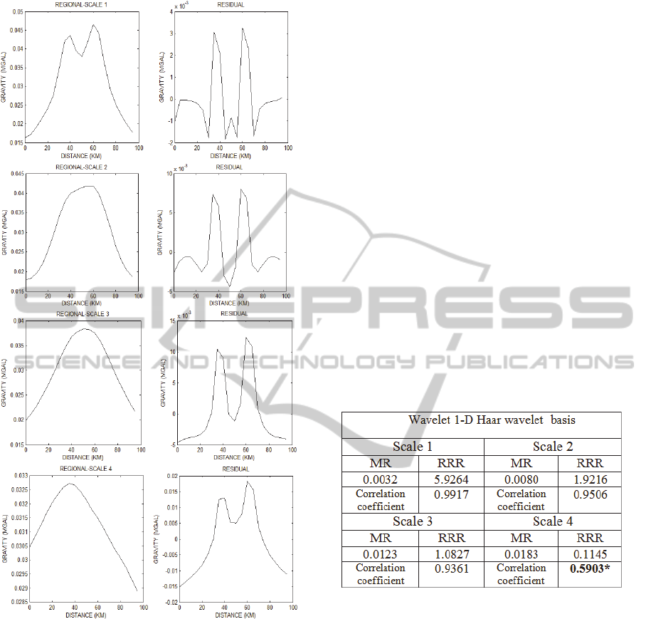
5.2 Separation of Real Data Due to
Cavity using Correlation
Coefficient Test
This real data which is located in west of Iran is due
to region that some other methods illustrate presence
of karstic phenomena (cavity) in it. From negative
anomalies which have been seen along each other, it
is found that the cavity has been located along the
north-south direction. Furthermore negative
anomalies which are correspondent to cavity are
discontinued at width of 215.5 m. this discontinuity
causes ambiguities in presence of cavity. The
proposed method in this study is used for data which
is led to results shown in Table 5.
Since values for RRR at scale 1 are less than unit
the minimum RRR test can not find the proper scale
for optimal wavelet application and then also
optimal separation. Less than unit RRRs indicate
original form distortion that vanish geologic
phenomenon which are accessible by appropriate
separated data. In this case, we choose the best scale
for residual effect removal by correlation coefficient
test.
a
b
Figure 5: a) Bouger map of original data. b) Cleaned
regional data in which a syncline is clearly detected.
Figure 6: it seems that there is a karstic phenomenon in
north-south direction. The dashed profile crosses the low
density zone vertically. There is no certain symptom of
low density in trend of data in that profile.
130 140 150 160 170 180
80
90
100
110
120
130
-0.3
-0.28
-0.26
-0.24
-0.22
-0.2
-0.18
-0.16
-0.14
-0.12
-0.1
-0.08
-0.06
-0.04
-0.02
0
0.02
0.04
0.06
0.08
0.1
0.12
0.14
0.16
130 140 150 160 170 180
80
90
100
110
120
130
-0.22
-0.2
-0.18
-0.16
-0.14
-0.12
-0.1
-0.08
-0.06
-0.04
-0.02
0
0.02
0.04
0.06
0.08
0.1
EffectiveResidualandRegionalGravityAnomalySeparation-Using1-D&2-DStationaryWaveletTransform
665
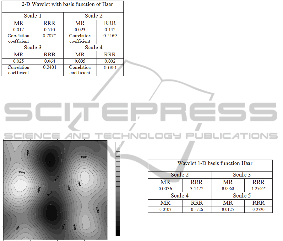
Table 5: Maximum residual and regional to residual ratio
and correlation coefficient provided by wavelet at
different scales for real data of cavity.
Because of large amplitude of residuals, from the
first step RRR of 2-D wavelet transformed images
are less than 1. Suitable scale is that its correlation
coefficient has not yet deviated form its decreasing
trend suddenly. Note that big scale and small RRR
test fails when their magnitudes are very small
because of extra big residuals.
Figure 7: regional map of data which has been shown at
Fig. 6. Appropriate scale is 1 and the proportional wavelet
function is dmey.
6 COMPARISON OF 1-D AND 2-D
WAVELET RESULTS FROM
SEPARATION PROCESSING
We used 1-D wavelet transform for separation of
data corresponds to profile as shown in Fig. 6.
According to the RRR test, Haar wavelet function at
scale 3 is known appropriate for maximum residual
separation; its result is offered at Table 6. The result
of 2-D wavelet which has been applied on data (for
comparison of 1 and 2-D results, the gravity trace of
the same profile has been selected from 2-D wavelet
map) indicates the application of scale 1 for
obtaining optimal separation is suitable.
We mean the same results as if both 1-D and 2-D
wavelet produce data which are geologically
interpreted the same and their trends are correlated
relatively. To check this we produce outputs
provided by wavelet at some more scales. Some
RRRs of various separation levels which provided
by both 1-D and 2-D wavelet at alternative scales are
less than unit which causes to be ignored them as
unacceptable geologic correlated tools for
separation. Therefore, we are able to prepare and
visualize transformed signal and map at any scale
but some of them suffer significant geologic and
geophysical interpretation. We use optimal results of
one and two dimensional by both tests to calibrate
the comparison and find out the relation in two
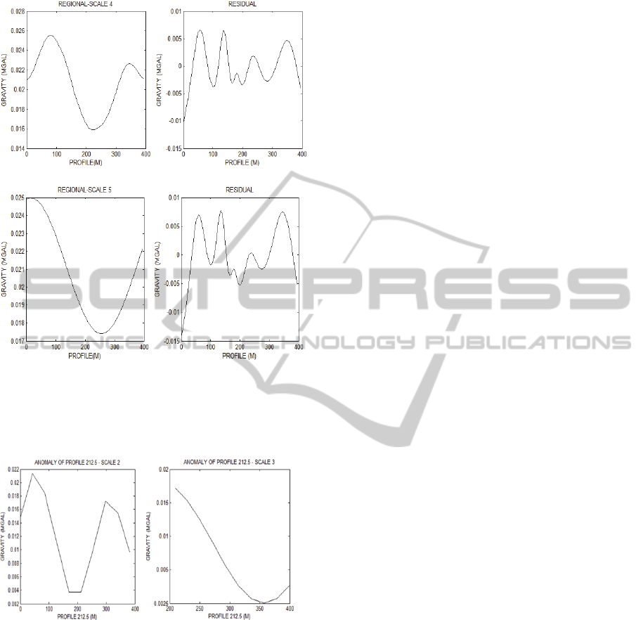
dimensions. Fig 8a and 8c are 1-D wavelet transform
of data due to profile shown at Fig. 6 at scales 4 and
5. Results of 2-D wavelet transform are brought in
Table 5 and are shown at Fig. 9.
Table 6: Maximum residuals, RRRs and correlation
coefficients for different scales provided for cavity.
Trends of regional portion by 1-D wavelet
transform at scales 4 and 5 are matched one by one
with proportional result of 2-D wavelet transform at
scales of 2 and 3. These anomalies are provided by
surface micro-anomalies; see b and d sections of Fig.
8. Since there are more stations (with smaller
intervals rather than other profiles) on individual
profile rather than other data acquiring lines, its
corresponding signal is smoother rather than ones
which are extracted from other grid lines of data.
Result at each scale of 2-D is proportional to ones by
1-D wavelet at scale with second next number. It
means 2-D wavelet at scale 1 is corresponding to 1-
D wavelet at scale 3 and so on. Finally, 2-D wavelet
at scale 1 and its corresponding 1-D wavelet at scale
3, show the path of cavity clearly.
0 50 100 150 200 250 300 350
0
50
100
150
200
250
300
350
-0.012
-0.01
-0.008
-0.006
-0.004
-0.002
0
0.002
0.004
0.006
0.008
0.01
0.012
0.014
0.016
0.018
0.02
0.022
0.024
ICPRAM2013-InternationalConferenceonPatternRecognitionApplicationsandMethods
666
a b
c d
Figure 8: a) 1-D wavelet transform at scales 4. b) Residual
reconstruction at scale 4. c) Result of application of 1-D
wavelet to data at scale 5. d) Residual reconstruction at
scale 5.
a b
Figure 9: a) Trend of data of profile like that in fig. 6,
correspond to regional map produced by 2-D wavelet
transform at scale 2. b) Trend of data of profile like that in
fig. 6, correspond to regional map produced by 2-D
wavelet transform at scale 3.
7 CONCLUSIONS
The residuals in gravity data which are due to
shallow micro-anomalies create high-frequency
effects in the original signal. Discrete stationary
wavelet transform was applied to separate them from
regional effect to clarify its trace. We want to
separate maximum residuals in amplitude that can be
interpreted as the biggest shallow anomalies.
Maximum scale which provides minimum and not
less than unit RRR has been determined for optimal
separation. We call this condition establishment of
RRR test that is introduced as credible technique for
maximum residual separation. If from the first scale
RRR is less than unit (this often happens in 2-D
wavelet) we choose the scale that correlation
coefficient has not still deviated from its decreasing
trend. Less than unit RRRs causes distortion of
regional signal or map from original form.
Application of test to synthetic gravity data
illustrated the usefulness of this technique for
maximum residual separation using above
mentioned tests. Separation of real data was led to
detect of syncline. 1-D and 2-D transforms was
applied on data of a Karstic area. We applied 2-D
wavelet transform using correlation coefficient test
that unmasked cavity (karst path) trace. It was seen
that 1-D wavelet results are similar with 2-D ones in
manner that 2-D wavelet at any scale is one by one
related to 1-D wavelet at second next scale (two
times). The advantage of wavelet is basis function
alternation that makes it possible to identify and
separate any shape and size micro-anomalies.
ACKNOWLEDGEMENTS
The first author would like to appreciate
encouraging guidance of Dr. H. Siah Koohi, at
University of Tehran for his valuable feedback
.
REFERENCES
Coifman, R. R., and Donoho, D. L., 1995: Translation-
invariant denoising, in Antoniadis, A., and
Oppenheim, G., Eds., Wavelets in statistics: Springer-
Verlag, 125–150.
Deng, X. Y., Yang, D. H., Peng, J. M., Guan, X., Yang, B.
J., 2011: Noise reduction and drift removal using
least-squares support vector regression with the
implicit bias term, Geophysics, Vol. 75, No. 6, pp.
V119–V127
Donoho, D. L., 1993: Nonlinear wavelet methods for
recovery of signals, densities, and spectra from
indirect and noisy data, in Daubechies, I., Ed.,
Different perspectives on wavelets: Proc. Symp. Appl.
Math, 47, 173–205.
Donoho, D. L. Johnstone I. M.,
1994: Ideal spatial
adaptation by wavelet shrinkage, Biometrika, Vol. 81,
pp.
425-455.
EffectiveResidualandRegionalGravityAnomalySeparation-Using1-D&2-DStationaryWaveletTransform
667

Fedi, M., Lenarduzzi,L., Primiceri, R., Quarta,T., 2000:
Localized Denoising Filtering Using the Wavelet
Transform Pure appl. geophys. VOL
157, pp 1463-
1491.
Fedi, M., Primiceri, R., Quarta, T., Villani, A. V., 2004:
Joint application of continuous and discrete wavelet
transform on gravity data to identify shallow and deep
sources, Geophys. J. Int. VOL
156, 7-21.
Leblanc, G. E., Morris, W. A., 2001, Denoising of
aeromagnetic data via the wavelet transform,
GEOPHYSICS, VOL.
66 NO. 6 , Pages 1793-1804.
Moreau, F., Gibert, D., Holschneider, M., and Saracco, G.,
1999: Identification of sources of potential fields with
the continuous wavelet transform: basic theory: J.
Geophys. Res., 104, B3, 5003–5013.
Neumann, M. H., and Von Sachs, R., 1995: Wavelet
thresholding beyond the Gaussian i.i.d. situation, in
Antoniadis, A., and Oppenheim, G., Eds.,Wavelets in
Statistics: Springer-Verlag, 301–329.
Ridsdill-Smith, T. A., and Dentith, M. C., 1999: The
wavelet transform in aeromagnetic processing:
Geophysics, 64, no. 4, 1003–1013.
Saito, N., 1994, Simultaneous noise suppression and
signal compression using a library of orthonormal
bases and the minimum description length criteria, in
Foufoula-Georgiou, E., and Kumar, P., Eds.,Wavelets
in geophysics: Academic Press, 299–324.
Soares, J. C., Tenorio, L., Li, Y. G.,
2004: “Efficient
automatic denoising of gravity gradiometry data,”
Geophysics, Vol.
69, No. 3, pp. 772-782.
Yan. P., Wu, Y.,
2011: Application of wavelet threshold
denoising method in
gravity data processing, IEEE,
International Conference on Multimedia Technology
(ICMT),pages
2972-2975.
Zou, C. C., Yang, X. D., Pan, L. Z., 1999: A new
technique for denoising log curve on the basis of
wavelet transform, Geophysical and Geochemical
Exploration, Vol. 23, No. 6, pp. 462–466.
ICPRAM2013-InternationalConferenceonPatternRecognitionApplicationsandMethods
668
