
Compensation of Unknown Input Dead Zone using
Equivalent-Input-Disturbance Approach
Liyu Ouyang
1,2
, Jinhua She
3
, Min Wu
1,2
and Hiroshi Hashimoto
4
1
School of Information Science and Engineering, Central South University, Changsha 410083, China
2
Hunan Engineering Laboratory for Advanced Control and Intelligent Automation, Changsha 410083, China
3
School of Computer Science, Tokyo University of Technology, Hachioji, Tokyo 192-0982, Japan
4
Master Program of Innovation for Design and Eng., Advanced Inst. of Industrial Tech.,
Shinagawa, Tokyo, 140-0011, Japan
Keywords: Compensation of Nonlinearity, Dead Zone, Distortion Factor, Equivalent Input Disturbance (EID),
Nonlinearity.
Abstract: This paper considers the problem of the compensation of an unknown dead zone in the input of a plant. A
new compensation method is presented based on the estimation of an equivalent input disturbance (EID).
Unlike other methods, this method does not require the exact information of a dead zone. First, we consider
the dead zone as an input-dependent disturbance and employ an EID estimator to estimate it. Then, we
incorporate the estimate in the control input and compensate the effect of the dead zone almost completely.
Simulation results demonstrate the validity of the method.
1 INTRODUCTION
Dead zone appears in many mechatronic systems,
for example, in a motor drive, a photoelectric sensor,
etc. This nonlinearity has a direct effect on the
accuracy of a controlled output and leads to the
deterioration of system performance (Hung et al.,
2008). The compensation of dead zone has attracted
considerable attention over the last few decades.
Many studies focused on a system with an
unknown dead zone in the control input. Since it is
very hard to precisely acquire the parameters of the
dead zone, it is difficult to completely compensate it,
and it causes a fundamental problem in high
precision control. To handle this nonlinearity, many
methods have been proposed for the case in which a
dead zone is measurable (Recker et al., 1991; Wang
et al., 2003). Tao and Kokotovic proposed a method
based on the construction of an adaptive dead zone
inverse for a system with an unmeasurable dead
zone (Tao and Kokotovic, 1994). However, their
method requires that the output of a dead zone is
within a known compact set. And the inverse model
of a dead zone is usually difficult to calculate. To
avoid the construction of an inverse model for a
dead zone, Ma and Yang (2008) proposed a new
adaptive control strategy. Since an adaptive control
method often causes the problem of instability, many
intelligent methods have been used to solve this
problem (Semilc and Lewis, 2000; Boulkroune and
M’saad, 2011). Sliding mode control was also used
to deal with nonlinearities in the control input by
making use of its fast switching speed (Tong and Li,
2003). But these methods are usually
computationally expensive and also have to meet the
matching condition.
In this paper, we present a new compensation
method for a plant with an unknown input dead zone.
Unlike other methods, this method is based on the
idea of an equivalent input disturbance (EID), which
was first presented by She et al. (2008) to deal with
the problem of disturbance rejection in a linear servo
system. The main advantages of this method are
1) It does not require any information of the
dead-zone.
2) The compensation effect is satisfactorily.
3) A robust control system can easily be designed
for the complemented plant using advanced
control theory, and high-precision tracking can
easily be achieved.
605
Ouyang L., She J., Wu M. and Hashimoto H..
Compensation of Unknown Input Dead Zone using Equivalent-Input-Disturbance Approach.
DOI: 10.5220/0004033706050609
In Proceedings of the 9th International Conference on Informatics in Control, Automation and Robotics (ICINCO-2012), pages 605-609
ISBN: 978-989-8565-21-1
Copyright
c
2012 SCITEPRESS (Science and Technology Publications, Lda.)
2 PROBLEM FORMULATION
We consider a single-input-single-output (SISO)
nonlinear plant. The linear part of the plant is
() () (),
() (),
d
xt Axt Bu t
yt Cxt
()
(
x
()
(
((
(1)
where
()
n
xt R
is the state,
Rty )(
is the
output, and
Rtu
d
)(
is the control input of the
linear part.
nn
AR
,
1
n
RB
, and
n
RC
1
.
d
u
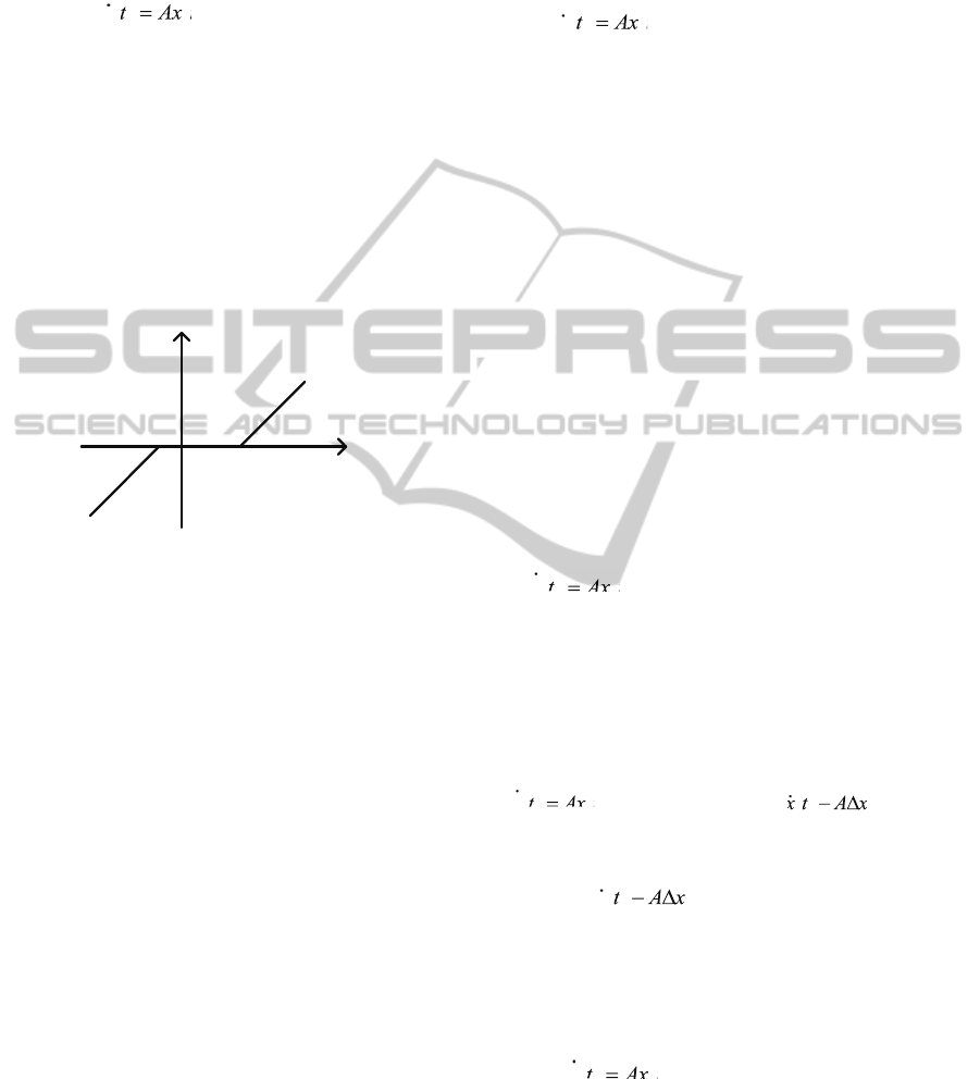
is the output of the input dead zone. It is described as
() , if () ,
() 0, if () ,
() , if () ,
rr
dlr
ll
ut b ut b
ut b ut b
ut b ut b
(2)
r
b
l
b
()ut
()
d
ut
Figure 1: Dead zone.
where (b
l
<0) and (b
r
>0) are the breakpoints of the
dead zone on the left- and right-half planes,
respectively (Fig. 1). And u(t) is the control input of
the plant.
We made the following assumptions.
Assumption 1: The linear part of the plant is a
minimum-phase system.
Assumption 2: The linear part of the plant is
controllable and observable.
Assumption 3: The output of the dead zone is
not measurable. The parameters, b
l
and b
r
, are
unknown.
Due to Assumption 3, we cannot construct an
inverse of the dead zone. In this study, we treat the
dead zone as an input-dependent disturbance
() () ( ()),
d
ut ut dut
(3)
where
,if () ,
( ( )) ( ), if ( ) ,
,if ().
rr
lr
ll
butb
dut ut b ut b
butb
(4)
(3) decomposes
()
d
ut
into a linear part,
ut
, and
a nonlinear part, d(u(t)). And d(u(t)) is an artificial
disturbance introduced in this study. Submitting (3)
into the state equation of (1) yields
() () () ( ())xt Axt But dut
()
(
xt Ax
()
(
)
((
(5)
To suppress the influence of the dead zone on the
output, we devise a mechanism to automatically
estimate and compensate d(u(t)) by employing an
EID estimator (She et al., 2008) in the next section.
3 DESIGN OF EID-BASED
COMPENSATOR
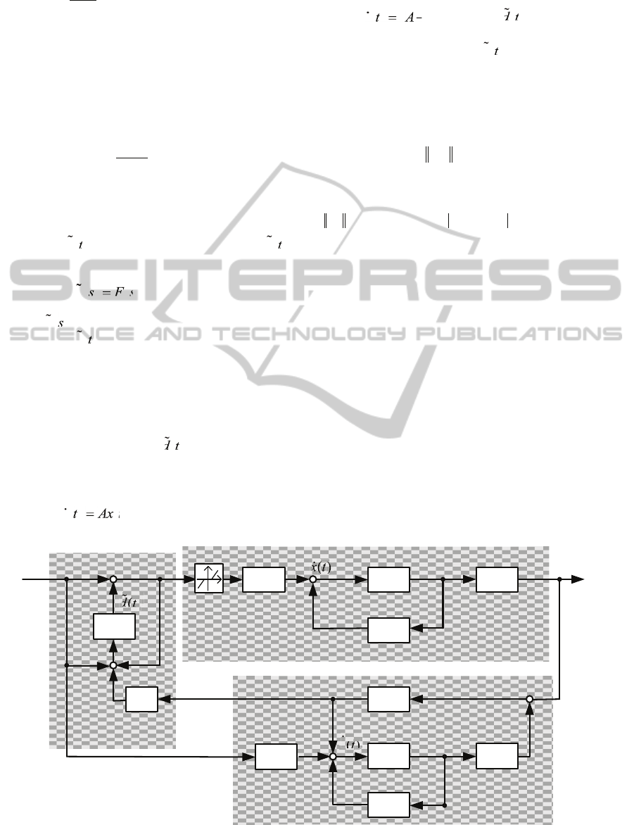
The configuration of the EID-based compensator for
dead zone is shown in Fig. 2. It has three parts: the
plant, a state observer, and an EID estimator.
3.1 Estimation of EID
To obtain an EID with high precision, we first
construct the following observer to reproduce the
state of the plant:
ˆˆ ˆ
() () () () (),
f
xt Axt Bu t L yt Cxt
ˆ
ˆ
() (
ˆ
x
ˆ
() ()
ˆ
((
(6)
where L is the observer gain.
Taking the error state to be
ˆ
() ()xxt xt
(7)
and substituting it into (5) yield
ˆˆ
() () () ( ()) () ()x t Ax t Bu t Bd u t x t A x t
ˆ
ˆ
xt Axt
ˆ
ˆ
() ()
ˆ
((
ˆ
()
()()
()()
(8)
We find a control input
()
e
dt
that satisfies
() () ()
e
xt A xt B d t
()
x
()
x
())
(9)
Combining (8) and (9) and denoting
ˆ
() ( ()) ()
e
dt dut d t
(10)
Give
ˆ
ˆˆ
() () () ()xt Axt B ut dt
ˆ
ˆ
x
Ax t
ˆ
ˆ
()
(
ˆ
(
(11)
From (6) and (11), we have
ˆ
ˆ
() ( () ()) () (),
f
dt B LCxt xt u t ut
(12)
ICINCO 2012 - 9th International Conference on Informatics in Control, Automation and Robotics
606
where
:
T
T
B
B
BB
.
ˆ
()dt
is an estimation of the
actual EID. From the above equations, we know that,
if the state of the observer is exactly equal to the state
of the actual plant, the estimated EID asymptotically
converges to the actual EID.
A low-pass filter
1
()
1
Fs
Ts
(13)
is used to select the angular-frequency band for the
disturbance estimate,
ˆ
()dt
. In (13), T is the time
constant of the filter. The filtered disturbance
estimate is
()dt
)
dt
(
. The relationship between
()dt
)
dt
(
and
ˆ
()dt
is
ˆ
() () (),Ds FsDs
()
(
D
()
(
)
(14)
where
()Ds
()
D
(
and
ˆ
()Ds
are the Laplace
Transform of
()dt
)
dt
(
and
ˆ
()dt
, respectively.
3.2 Design of Filter and State Observer
(12) equals to
ˆ
() () ()dt BLC xt dt
)
d
(
(
(15)
If there is no nonlinearity, the plant (5) is
() () ()xt Axt But
() (
x
()
(
((
(16)
And
() ( ) () ()xt A LC xt Bdt
)
d
((
() (
xt A
() ()(
x
() ()(
(
(17)
The transfer function from
()dt
)
dt
(
to
ˆ
()dt
is
1
()( )Gs B sI A sI A LC B
(18)
From the small-gain theorem, we know that
1GF
(19)
guarantees the stability of the estimation, where
:sup ()()
max
0
GF G j F j
and
max
()j
is
the maximum singular value of
G
.
From Assumption 1, we know that the dual
system
(,, )
TTT
ABC
is also a minimum-phase
system. The concept of perfect regulation shows that
a very large weighting parameter,
, in a quadratic
performance index ensures
1
lim ( ) 0
TTT
BsI A CL
(20)
Since the left side of this equation is part of the
transfer function,
()Gs
, (18) and (20) mean that a
large enough
makes the condition (19) true.
B
A
1
sI
()Fs
B
1
sI
L
B
A
C
C
()yt
()xt
ˆ
()xt
ˆ
()xt
ˆ
ˆ
()
x
ˆ
()yt
State
observer
Plant
Disturbance
estimator
()dt
)
ˆ
()dt
()
f
ut
()ut
()xt
Figure 2: Configuration of EID-based compensator for dead zone.
Compensation of Unknown Input Dead Zone using Equivalent-Input-Disturbance Approach
607
4 NUMERICAL EXAMPLE
Consider the nonlinear plant, (1) and (2), with:
11
10
A
,
1
0
B
,
01C
,
(21)
1
l
b
,
1
r
b
.
(22)
We chose
0.05T
s and the input as
5sin 2 /
fs
utT
, T
s
= 2 s.
(23)
Using MATLAB function, lqr to solve
!
9
0,
=diag 10 ,1 , 1
TT T
PA A P PC CP Q
Q
(24)
Yielded
31371 250
T
LPC
(25)
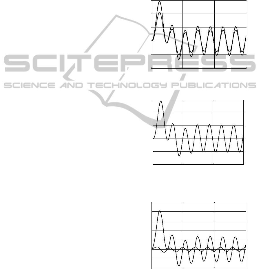
The simulation results are shown in Figs. 3-5. It is
clear from Fig. 3 that the effect of the dead zone on
the output of the plant cannot be ignored. Fig. 4
shows the EID-based compensation results.
Comparing Fig. 4 with Fig. 3, we can see that the
EID-based compensator reduced the effect of the
dead zone on the output greatly and the output of the
compensated nonlinear plant is almost the same as
that of the plant without the input dead zone. When
the dead zone was not compensated, the largest error
between the outputs of the plant without the dead
zone and with the dead zone was 0.4. On the other
hand, it reduced to 0.027 when the EID-based
compensator was used.
To assess the effectiveness of the EID-based
compensation method, a comparison was made
between two outputs for a sine wave input. One is
the output of the plant without the dead zone, and
the other is the output of the EID-based
compensated plant with the dead zone. Three
characteristic factors (Kim & Russell, 1995) were
calculated (Tab. 1). Clearly, the distorted output
caused by the dead zone was compensated almost
completely.
5 CONCLUSIONS
A dead zone often exists in mechatronic systems. It
deteriorates the control performance. In this paper,
we presented an EID-based compensation method
for a plant with an unknown input dead zone. We
regarded the dead zone nonlinearity as an
input-dependent disturbance, estimated an EID, and
added it to the input channel. This method does not
need any information of the dead zone. We do not
need to calculate an inverse dynamics of the dead
0 5 10 15
-1
-0.5
0
0.5
1
1.5
time(s)
output
----b
----a
b----with dead-zone
a----without dead-zone
Figure 3: Outputs of plant with and without dead zone.
0 5 10 15
-1
-0.5
0
0.5
1
1.5
time(s)
output
Figure 4: output of plant with dead zone using EID-based
compensator.
0 5 10 15
-0.2
-0.1
0
0.1
0.2
0.3
0.4
0.5
a--without compensation
b--with compensation
----a
----b
time
(
s
)
output error
Figure 5: Output errors of plant with and without using
EID-based compensator.
ICINCO 2012 - 9th International Conference on Informatics in Control, Automation and Robotics
608

Table 1: Comparison of characteristic factors of outputs.
Form
factor
Crest
f
actor
Dist
ortion
factor
Without dead zone
1.114
1.414
0
With compensation
1.113
1.41
5
0.021
zone as well. Simulation results show that this
method provides good compensation performance.
ACKNOWLEDGEMENTS
The work of L. Ouyang and M. Wu was supported
by the National Science Foundation of China under
grants 60974045 and 60674016. And the work of J.
She and H. Hashimoto was supported by Casio
Science Promotion Foundation.
REFERENCES
Boulkroune, A. & M’saad, M., 2011. A practical
projective synchronization approach for uncertain
chaotic systems with dead-zone input.
Communications in Nonlinear Science and Numerical
Simulation, 16, 4487-4500.
Hung, Y. C., Yan, J. J. & Liao T. L., 2008. Projection
synchronization of chua’s chaotic systems with
dead-zone in the control input. Math Computer
Simulation, 77, 374-382.
Kim, C. J. & Russell, B. D., 1995. Analysis of distribution
disturbances and arcing faults using the crest factor.
Electric Power Systems Research, 35, 141-148.
Ma, H. J. & Yang, G. H., 2008. Adaptive regulation of
uncertain nonlinear systems with dead-zone.
Proceedings of the 47th IEEE Conference on Decision
and Control Cancun, 1950-1955.
Recker, D. A., Kokotovic, P. V., Rhode, D. & Winkelman,
J., 1991. Adaptive nonlinear control of systems
containing a dead-zone. Proceedings of the 30th
Conference on Decision and Control. 1991,
2111-2115.
Selmic, R. R. & Lewis, F. L., 2000. Dead-zone
compensation in motion control systems using neural
networks. IEEE Transactions on Automatic Control,
45 (4), 602-613.
She, J., Fang, M., Ohyama, Y., Hashimoto, H, & Wu M.,
2008. Improving disturbance-rejection performance
based on an equivalent-input-disturbance approach.
IEEE Transactions on Industrial and Electronics, 55,
380-389.
Tao, G. & Kokotovic, P. V., 1994. Adaptive sliding
control of plants with unknown dead-zone. IEEE
Transactions on Automatic Control, 39 (1), 59-68.
Tong, S. & Li H. X., 2003. Fuzzy adaptive sliding-mode
control for MIMO nonlinear systems. IEEE
Transactions on Fuzzy Syst., 11 (3), 354-360.
Wang, X. S., Hong, H. & Su, C. Y., 2003. Model
reference adaptive control of continuous time systems
with an unknown dead-zone. IEE
Proceedings-Control Theory and Applications, 150 (3),
261-266.
Compensation of Unknown Input Dead Zone using Equivalent-Input-Disturbance Approach
609
