A CONTROL PARADIGM FOR DECOUPLED OPERATION

OF MOBILE ROBOTS IN REMOTE ENVIRONMENTS

Remo Pillat, Arjun Nagendran and Charles E. Hughes

Synthetic Reality Lab, University of Central Florida, 3100 Technology Pkwy, 32826, Orlando, FL, U.S.A.

Keywords:

Mobile Robots, Tele-operation, Virtual Environments, Robot Simulation.

Abstract:

Remote operation of robots in distant environments presents a signiﬁcant challenge for direct control due

to inherent issues with latency and available bandwidth. Purely autonomous behaviors in such environments

come with the associated risks of failure. It may be advantageous to acquire information about the environment

from the robot’s onboard sensors, to re-create a simulation and plan a mission beforehand. The planned

mission can then be uploaded to the robot for execution, allowing the physical robot to handle the autonomy

required for completing its task. In this paper, the foundations of a control paradigm are presented that uses

a simulated virtual environment to decouple the operator from the physical robot, thus circumventing latency

problems. To achieve this, it is ﬁrst required to accurately model the robot’s kinematic parameters for use in

the simulation. Kalman ﬁltering techniques that demonstrate this modeling for a differential drive robot are

presented in this paper. The estimated parameters are then used as inputs to a modular planning and execution

module. Based on simulation results, a safe and non-redundant path can then be uploaded and executed on the

real robot.

1 INTRODUCTION

Robots have become a ubiquitous presence in today’s

society. They have found uses in diverse areas such

as manufacturing, health care, planetary exploration,

and entertainment. Autonomous operation of these

robots is usually limited to processes that occur in

controlled environments and involve repetitive steps,

e.g. the assembly of cars.

Whenever a robot is deployed on a remote mis-

sion, some form of tele-operation has to be employed.

Conventionally, tele-operation refers to the direct con-

trol of a robot from a remote location using onboard

sensors that provide the required navigational aids. In

mobile robotics this need is most pronounced in ex-

ploring areas that are hazardous or inaccessible to hu-

mans, e.g. when surveying a stricken nuclear plant

or controlling a rover on a different planet. Recently,

the medical community has made long strides towards

making minimally invasive robotic surgery a routine

procedure, but in most commercially available sys-

tems the operator has to be located in close physical

proximity. Remote tele-operation is however always

hampered by the inescapable bandwidth limitations

and communication time delays (latency).

Transmission delays and bandwidth limitation are

an unavoidable feature of long-distance communica-

tion. These must be compensated for within existing

control schemes or an alternative control paradigm

must be applied. In this work, an architecture will be

presented that decouples the operator’s actions (mas-

ter) on a simulated robot from the executed actions on

the real robot (slave) through a virtual reality-based

simulation layer. The general control paradigm is

based on the following assumptions that are not pre-

sented in the scope of this paper.

• The simulation environment can be constructed

by gathering real-world data through the robot’s

onboard sensors and is sufﬁciently representative

within a localized region around the robot.

• The real robot has sufﬁcient autonomy to be able

to execute a mission plan under the inﬂuence of

external uncertainties, or report discrepancies that

prevent execution.

An operator can work in the simulation environment

to plan and execute his mission either by controlling

the robot manually, or experiment with higher level

autonomous planning modules. Once mission execu-

tion in simulation is completed, a set of modules pro-

cess the simulation data to re-create a mission plan

for the real robot. The modules are capable of accept-

ing user inputs to prioritize the mission’s goals and

553

Pillat R., Nagendran A. and E. Hughes C. (2012).

A CONTROL PARADIGM FOR DECOUPLED OPERATION OF MOBILE ROBOTS IN REMOTE ENVIRONMENTS.

In Proceedings of the International Conference on Computer Graphics Theory and Applications, pages 553-561

DOI: 10.5220/0003947205530561

 SciTePress

remove any redundancy in the simulated mission. A

newly created mission plan is then uploaded to the

real robot for execution. The work presented herein

focuses on the use of Kalman ﬁltering techniques to

determine the robot’s kinematic parameters and the

role of the different modules in the decoupling pro-

cess.

2 BACKGROUND

Traditionally, bilateral tele-operation with time delays

requires specialized control schemes to assure sys-

tem stability and transparency. Good surveys of these

methods can be found in (Arcara and Melchiorri,

2002) and (Hokayem and Spong, 2006).

All of these methods try to address the problem

of direct control of the slave by the master under the

presence of time delay. If the time delays are highly

variable or impractical to the operators other methods

have to employed. (Pan et al., 2006) takes a new ap-

proach be proposing a dual predictor/observer control

schemes on both the master as well as the slave side,

thus circumventing the usage of any delayed informa-

tion.

In one of the earliest attempts for an alternative

paradigm, (Bejczy et al., 1990) displays a virtual

”phantom robot” on the master side that can be con-

trolled directly without time delay. In these experi-

ments the real robot arm follows the phantom move-

ments with the implicit time delay. Unfortunately,

this scheme increases the execution time of any mo-

tion, because the operator will perform a motion on

the phantom robot and then has to wait until the real

robot attains the same conﬁguration. (Kheddar, 2001)

ﬁrst introduced the ”hidden robot concept” that com-

pletely abstracted the movements of the real robot

from the operator by only presenting him with a vir-

tual presentation.

(Kheddar et al., 2007) provides a more recent sur-

vey of the state-of-the-art in using virtual reality sim-

ulations to overcome the inherent tele-operation lim-

itations. Closely related to our work is the emerg-

ing ﬁeld of Teleprogramming (Hernando and Gam-

bao, 2007) where the operator does not directly con-

trol the robot, but a simulated copy. After an action is

executed, an abstract command sequence that signals

operator intent is sent to the slave robot. The authors

make an effort to abstract the underlying system vari-

ables on the master and slave side and only transmit

operator intentions. This approach is laudable in its

generalizing power, but has implicit requirements of

accurate simulation models for robots and the envi-

ronment.

With exception of (Wright et al., 2006) and (Yu

et al., 2009), many teleprogramming systems focus

on the operation of robot arms, while systems tailored

towards mobile robot tele-operation have gained less

attention. This might be due to the fact that the phys-

ical simulation of mobile robots dynamics and envi-

ronment interaction is non-trivial.

Professional robot simulators have sufﬁciently ad-

vanced to provide a satisfactory simulation of physi-

cal interactions between robot and the environment.

Examples of commercial systems include Marilou

(Anykode, 2011), Webots (Michel, 2004), and Mi-

crosoft Robotics Studio (Jackson, 2007).

Predictive simulators have also been used to allow

multi-robot coordinating missions as in (Chong et al.,

2000).

3 SYSTEM ARCHITECTURE

As stated previously, transmission delays, missing

communication packets, and bandwidth limitation are

an unavoidable feature of long-distance communica-

tion. Communication latencies beyond several hun-

dred milliseconds are generally unacceptable for hu-

man operators and produce dangerous control insta-

bilities. This paper proposes an architecture that

decouples the operator’s actions from the executed

motions of the robot. This has several advantages

that can not be achieved in traditional tele-operation.

Given a representation of the environment, operators

can plan and execute simulated missions without the

need for a permanent communication connection to

the physical robot. Time-intensive trial runs can be

shortened, while invalid inputs and redundancies can

be corrected before any commands are uploaded to

the real robot.

The general control infrastructure will support

both goals of visual and operational ﬁdelity on the

master’s side as well as tight closed-loop control with-

out time delay by the slave (Figure 1).

At the highest level, our Master-Slave Control Ar-

chitecture (Zhu et al., 2011) features a simulation

server that maintains an environmental model and

simulated robotic entities with sensors and actuators.

All simulation components are based on the com-

mercial Marilou robotics simulator (Anykode, 2011).

Without a physical complement, a program can be

launched locally that controls the movements of the

robot in the simulated environment. This is the master

layer and it can function independently of any other

communication.

The uniqueness of the control architecture lies

in decoupling the networked layers. The simulation

GRAPP 2012 - International Conference on Computer Graphics Theory and Applications

554

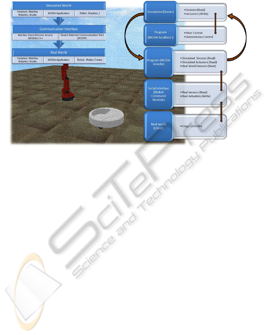
Figure 1: General architecture of the control paradigm.

layer is used to plan and execute movements before-

hand. These planned movements guide the real robot

that attempts to closely follow the simulated robot

without the need for explicit user control, while main-

taining a degree of autonomy to cope with dynami-

cally changing situations.

A remote program residing on the slave in the

real world connects to the Master and reads the val-

ues from the simulated sensors / actuators. The com-

munication interface then translates the actuator com-

mands to the real-robot (slave). At the same time,

real world sensors are read and data is fed back to

the simulation establishing a bilateral communication

interface; discrepancy in the received data from that

predicted by the simulation causes control to be trans-

ferred back to the Master.

The strength of the presented system, in compari-

son to the predictive simulation systems mentioned in

section 2, is its inherent ability to initially identify and

continually update the simulated representation of the

robot. Previous work relied heavily on a priori avail-

able simulation models or overly simpliﬁed physical

modeling. In addition, the modularity of the archi-

tecture allows easy addition of high-level planning or

processing modules.

While interpreting sensor data to recreate a simu-

lation dynamically forms one component, it is equally

important to have a robust model of the robot itself

in the simulation. Section 4 will focus on the use

of Kalman ﬁltering techniques to estimate the robot’s

kinematic parameters for use in simulation. These es-

timates are then passed as inputs to the modular plan-

ning and execution system which processes the simu-

lated data to generate a feasible mission plan for the

real robot (see Section 5). The signiﬁcance of estima-

tion errors in these parameters on the simulation are

highlighted in Section 6.

4 KINEMATIC ROBOT

SIMULATION MODEL

An accurate kinematic model of the controlled entity

is essential for any predictive simulation of robot mo-

tions. The existence and accuracy of this model is an a

priori requirement for both the validity of the physical

simulation in the master virtual environment as well

as the legitimacy of any simulated planning action.

In existing systems that demonstrated the tele-

operation of mobile robots, for example (Yu et al.,

2009) and (Wright et al., 2006), this robot model is as-

sumed to be provided to the simulator with sufﬁcient

accuracy. In most cases, the parameters of this model

are hard to quantify, because values from manufac-

turer’s speciﬁcations or manual measurements are ei-

ther non-existent, prone to errors, or can vary from

one robot to the next. Through the example in Sec-

tion 6 it will be convincingly argued that even small

changes of the robot’s kinematic variables have a str-

A CONTROL PARADIGM FOR DECOUPLED OPERATION OF MOBILE ROBOTS IN REMOTE ENVIRONMENTS

555

ong inﬂuence on the accuracy of the motion simula-

tion in the planning and execution stages. For any

system employing a simulated mobile robot, this fact

cannot be overstated, because in the overall system ar-

chitecture many higher level modules will depend on

the precision of the kinematic parameters.

This makes the need for an automatic calibra-

tion method more pronounced. In this section, the

kinematic model of the well-known differential drive

conﬁguration will be developed. In addition, a uni-

ﬁed framework for the automatic identiﬁcation of the

kinematic parameters of a differential-drive robot will

be presented that allows off-line as well as online es-

timation. Ideally, this process will be self-calibrating

and should not require any human control input be-

yond a rough initial value of the estimated entities.

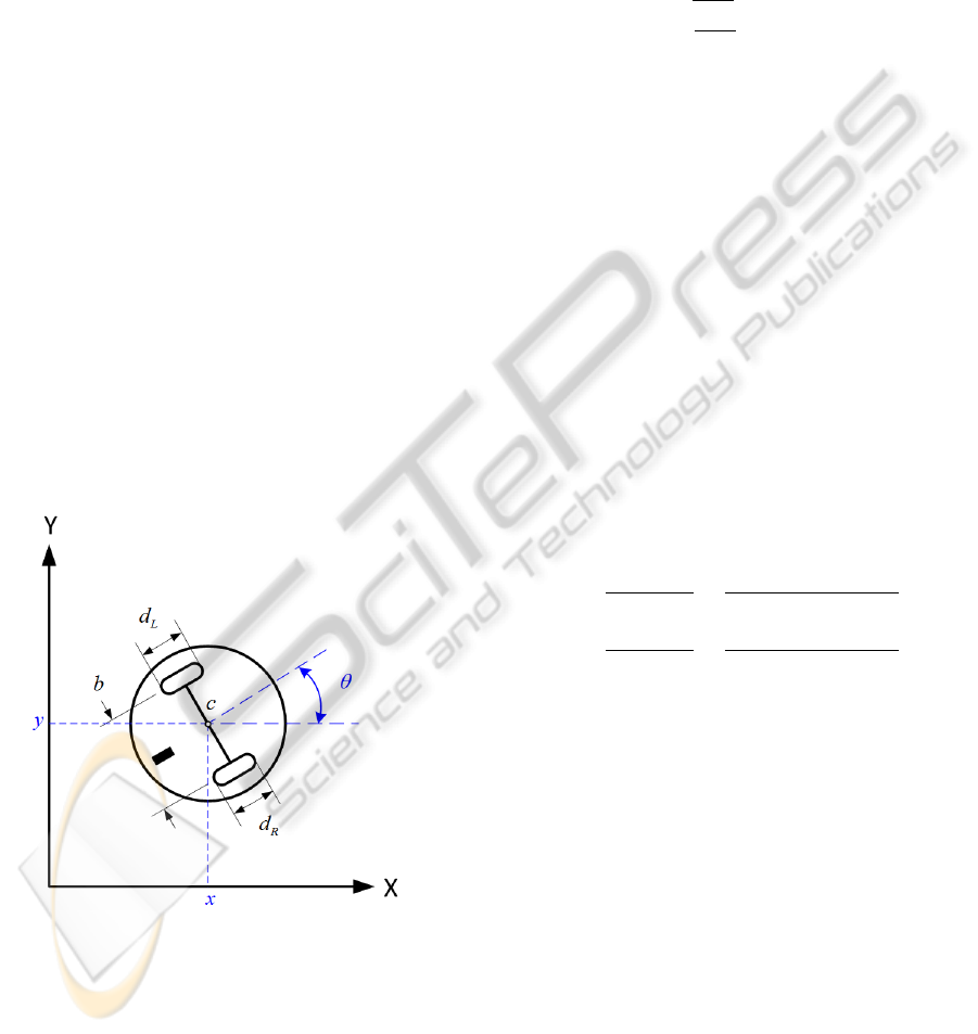
4.1 Basic Differential Drive Model

The differential drive conﬁguration is a commonly en-

countered mobile robot combination that uses two ac-

tuated wheels and one or more (passive) casters. For

the purposes of this work the parameters of this con-

ﬁguration can be simpliﬁed according to Figure 2.

The kinematic parameters that should be esti-

mated are the diameters of the left and right wheels

and d

, respectively), and the wheel base b.

Figure 2: Differential drive conﬁguration. Here d

and d

denote the diameters of the left and right wheel, respec-

tively. c is the center point between the actuated wheels

and b is the wheelbase.

When the robot moves in 2D its basic state at time

instant k can be described by x = [x,y, θ]

. Here the

coordinates (x,y) denote its position and θ the orien-

tation of its body.

Depending on the sampling time, the movement of

a differential drive robot can be approximated either

by a linear motion or, more generally, a circular arc.

Following the derivation for the latter case outlined in

(Wang, 1988), the state transition between time steps

k and k + 1 can be described as follows:

x =





k−1









sin(α)

∆s cos(θ

k−1

+ α)

sin(α)

∆s sin(θ

k−1

+ α)

∆θ





(1)

Here ∆s denotes the distance that the center c of

the robot traverses along the circular arc. The change

in orientation is signiﬁed by ∆θ

. α = ∆θ

/2 is simply

the half angle of the orientation change.

4.2 Incorporating Odometry Readings

In most cases, the odometry of the robot is derived

from encoders that are mounted on the driveshaft of

the actuated wheels. Even if they are not equipped on

a mobile base, they can easily be retroﬁtted.

Let e

res

be the encoder resolution per wheel rota-

tion. This value is constant and assumed to be known.

The encoder count differences between time steps are

indicated by ∆e

for the left wheel and ∆e

for the

right one.

Then the values for ∆s and ∆θ in Equation (1) can

be reformulated (under no wheel-slip conditions) as:

∆s =

∆s

+ ∆s

π (d

∆e

+ d

∆e

)

2 e

res

(2)

∆θ =

∆s

− ∆s

π (d

∆e

− d

∆e

)

res

(3)

∆s

is the distance traveled by the left wheel and

∆s

the equivalent quantity for the right wheel.

These derived equations will be used for estimat-

ing the state of the robot between time steps. Because

the robot state depends on our kinematic unknowns,

they can be estimated continuously while the robot

drives an arbitrary path.

4.3 Online Estimation

For estimating the state of a linear system, the Kalman

Filter (Kalman, 1960) and its many derivatives have

been the de facto standard in the robotics commu-

nity. Under the assumption that all state variables are

perturbed by zero-mean normal-distributed noise, the

Kalman Filter is an optimal recursive estimator for the

state variables of linear dynamical systems.

As can readily be seen by inspecting Equation (1),

the state transition between samples is described by

GRAPP 2012 - International Conference on Computer Graphics Theory and Applications

556

nonlinear equations. To handle that, this paper will

use the Extended Kalman Filter (Julier and Uhlmann,

2004), which linearizes the state transition equations

around the current mean and covariances of the esti-

mated quantities.

Akin to the state description in Section 4.1, our

state vector is x, but the process is now governed by

the non-linear function f :

= f (x

k−1

) (4)

Here, the non-linear function f relates the state

k−1

from the last time step and process noise w

∼

N(0,Q) to the current state.

A vector of measurements can be calculated by:

= h(x

) (5)

Here, the non-linear function h relates the a priori

state x

and measurement noise v

∼ N(0, R) to the

expected measurements z

In the update step of the ﬁlter, external measure-

ments of the robot state need to be integrated into the

current estimate. For the purposes of the experiments

presented here, the absolute position and orientation

of the robot is measured through an external optical

tracking system by Optitrack. Alternatively, a scan

matching based approach with a mounted laser scan-

ner could be used.

4.4 Augmented Extended Kalman Filter

The state vector x = [x,y,θ]

can be used to estimate

the pose of the robot based on internal encoder and

external tracking readings as outlined in Section 4.3.

If the values of the wheel diameters d

and d

and

the wheel base b are known only approximately or

are variable during robot operation, systematic errors

will be injected into the estimation process. This will

invariably lead to a degradation of Kalman Filter per-

formance. Examples of systematic errors include un-

equal wheel diameters, wheel misalignment, and ef-

fective wheel base ambiguities due to non-point ﬂoor

contact.

To alleviate that, the ideas from (Larsen, 1998)

and (Martinelli et al., 2007) can be followed to aug-

ment the state vector by the unknown quantities. De-

viating from this previous work, the wheel diameters

and wheel base are added directly to the state vec-

tor instead of using an artiﬁcial multiplier. The aug-

mented state vector is thus

x = [x,y,θ,d

,b]

(6)

The linearized (6x6) system matrix can be derived

based on the Jacobians of the non-linear function f in

Equation (4). The partial derivatives can be readily

found through symbolic differentiation in Matlab.

4.5 Experimental Validation

To validate the usefulness of the ﬁlter proposed in

Section 4.4, the robot is driven multiple times along a

circular path with a set of predetermined wheel veloc-

ities. Encoder readings of both wheels are recorded at

20 ms intervals.

The absolute position and orientation of the robot

is determined by a mounted marker pattern that is

tracked by an infrared camera system. The optical

tracking data was logged and served as ground truth

for this test run.

The test is performed at relatively slow speeds, so

wheel slippage on the surface can be ignored. After

the run concludes, the Augmented EKF is executed

off-line on the log data. For the purposes of this evalu-

ation, only the mean estimated values for wheel diam-

eters d

and d

and wheel base b are used for further

calculations.

As a baseline, d

, d

, and b were measured man-

ually and the robot path was calculated through the

dead reckoning equations ( Equation (1) and Equa-

tion (2)). One would expect the shape of the resulting

circle to closely resemble the shape recorded by the

optical tracker.

To each set of circles, an ellipse was ﬁtted and

its measurements for major axis, minor axis and area

were used as indicators for the validity of the esti-

mated parameters. Table 1 shows the results of this

run.

Table 1: The robot is driven along a circular path. Tracking

data is collected and a dead-reckoned path is calculated for

different values of wheel diameters and wheel base. The

”Baseline” is measured manually (d

= d

= 6.44 cm, b =

26 cm), while the ”Calibration” values are the mean output

of the Augmented Extended Kalman Filter (d

= 4.647 cm,

= 4.517 cm, b = 26.98 cm).

Major Axis a Minor Axis b Ellipse Area

(in cm) (in cm) (in cm

)

Tracking Data 107.714 107.44 9089.235

(Ground Truth)

Dead Reckoning 109.875 109.036 9409.337

(Baseline)

Dead Reckoning 107.101 106.387 8948.930

(Calibration)

Clearly, the quality of the dead reckoning im-

proves with the newly calibrated values. This bodes

well for the integration of the calibration into the vir-

tual reality simulation of the mobile robot.

Although this experiment was performed off-line

for convenience, the Kalman ﬁlter is designed to ex-

ecute online while the robot is running and continu-

ously update its estimates.

A CONTROL PARADIGM FOR DECOUPLED OPERATION OF MOBILE ROBOTS IN REMOTE ENVIRONMENTS

557

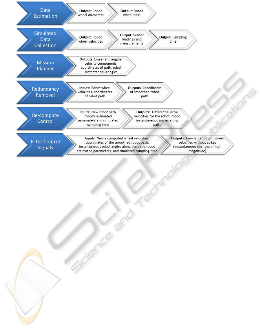
Figure 3: Planning and execution modules.

5 PLANNING AND EXECUTION

IN SIMULATION

The planning and execution stage is used on the mas-

ter (simulation) side of the tele-operation to allow the

operator to explore planning strategies and preview

anticipated robot movements. This stage is divided

into modules that are processed sequentially until a

ﬁnal successful behavior can be implemented on the

real robot. Figure 3 depicts the six modules used

during planning and execution, highlighting the in-

puts and outputs of each module. The absence of an

explicit input indicates that this information directly

ﬂows in from the outputs of the module above it.

Data Estimation: The data estimation module is

implemented according to the description in Section 4

i.e. the robot wheel diameters and wheel base are es-

timated using a Kalman Filter.

Simulated Data Collection: The data collection

module logs all simulated data during a mission, in-

cluding sampling time, left and right wheel velocities

of the robot, encoder counts, and all readings of the

mounted sensors.

Mission Planner: The mission planner integrates

the estimated and simulated data to re-create the exe-

cuted mission including generation of the coordinates

of the robot path that must be passed as an input to the

redundancy removal module.

Redundancy Removal: This module initializes

regions of interest based on the deﬁnition of redun-

dancy (user-speciﬁed). A matrix of distances between

the coordinates on the redundant path is used to ﬁnd

pinch points (intersecting points) across the curves.

These pinch points are used to delete any kinks or

loops in the robot path, which are redundant.

Re-compute Control: The new path (time-series)

is used to regenerate velocity vectors for the robot i.e.

individual wheel velocities for the differential drive

steering mechanism are re-computed based on the de-

sired linear and angular velocities.

Filter Control Signals: The deletion of segments

in the original path may result in the new path requir-

ing instantaneous changes in robot velocity, leading to

spikes in the control signal for each wheel. As a result

of this deletion, the robot might be expected to be in a

new position at the next sampling instant that is phys-

ically infeasible to attain. The path must therefore

be re-interpolated between the regions where spikes

occur, resulting in smoothed control signals for each

robot wheel. For every control signal spike, the path

of the robot is interpolated by increasing the travel-

time between the spike-points. This involves a re-

sampling of the position and velocity vectors of the

GRAPP 2012 - International Conference on Computer Graphics Theory and Applications

558

robot to increase overall time for the mission. The

orientation of the robot must be interpolated sepa-

rately since simultaneous changes in position and ori-

entation of the robot can occur during the removal

of kinks. Magnitude of velocity and angular veloc-

ity of robot are together used to determine left and

right wheel velocities. The process is also iterative

for each spike in the list, since the newly computed

values for position and orientation are re-used in the

interpolation process.

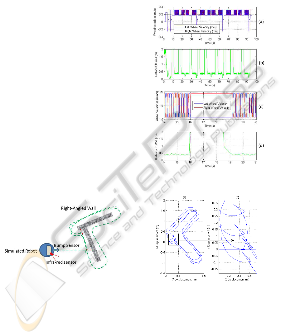
5.1 Case Study: Simple Wall Following

Routine

A simulation scenario was created with a right-angled

wall in the center of an indoor environment as shown

in Figure 4. The simulated robot had a single infrared

sensor mounted at its side at an acute angle, and a

bump sensor. The robot utilized a differential drive

steering and was programmed to perform a simple

wall following routine. When the bump sensor was

triggered on contact, it would cause the robot to re-

verse; following which it turned to its left and moved

along the wall using a loosely tuned proportional con-

troller acting on the error from the desired wall dis-

tance. The green dotted lines in the depiction indi-

cate a rough path that the robot would follow when

this algorithm was used. The red dots indicate regions

where the robot would have to back up since the bump

sensor was triggered.

Figure 4: Simulation setup.

Figure 5(a) shows the left and right wheel veloc-

ities during the wall following routine. Figure 5 (b)

shows the distance to the wall as measured by the

on-board infrared sensor. A section of both graphs

is magniﬁed for closer examination (Figure 5(c) and

Figure 5(d)). The data is generated by combining the

data estimation and simulated data collection mod-

ules. The continuous oscillations to compensate for

the wall distance-error highlights the implementation

of the proportional controller. Notice that the high

values of wall distance result in a corresponding dif-

ference in wheel velocities causing the robot to turn

in an arc until the infrared sensor picks up the wall

again.

Figure 5: Wall distance and wheel velocities. The graphs

are described in detail in Section 5.1.

Figure 6: Path of robot during wall-following.

Figure 6 (a) shows the actual path of the robot

around the right-angled wall in the simulation. This

is generated by the mission planner module. A por-

tion of Figure 6 (a) has been zoomed into in Figure 6

(b) to show the redundant traversal of paths by the

simulated robot. This occurs when the bump sensor

makes contact with the wall and the robot backs up

before turning away. In this case, redundancy is de-

ﬁned as a portion of the path that can be eliminated

from the simulated path, without causing a change

A CONTROL PARADIGM FOR DECOUPLED OPERATION OF MOBILE ROBOTS IN REMOTE ENVIRONMENTS

559

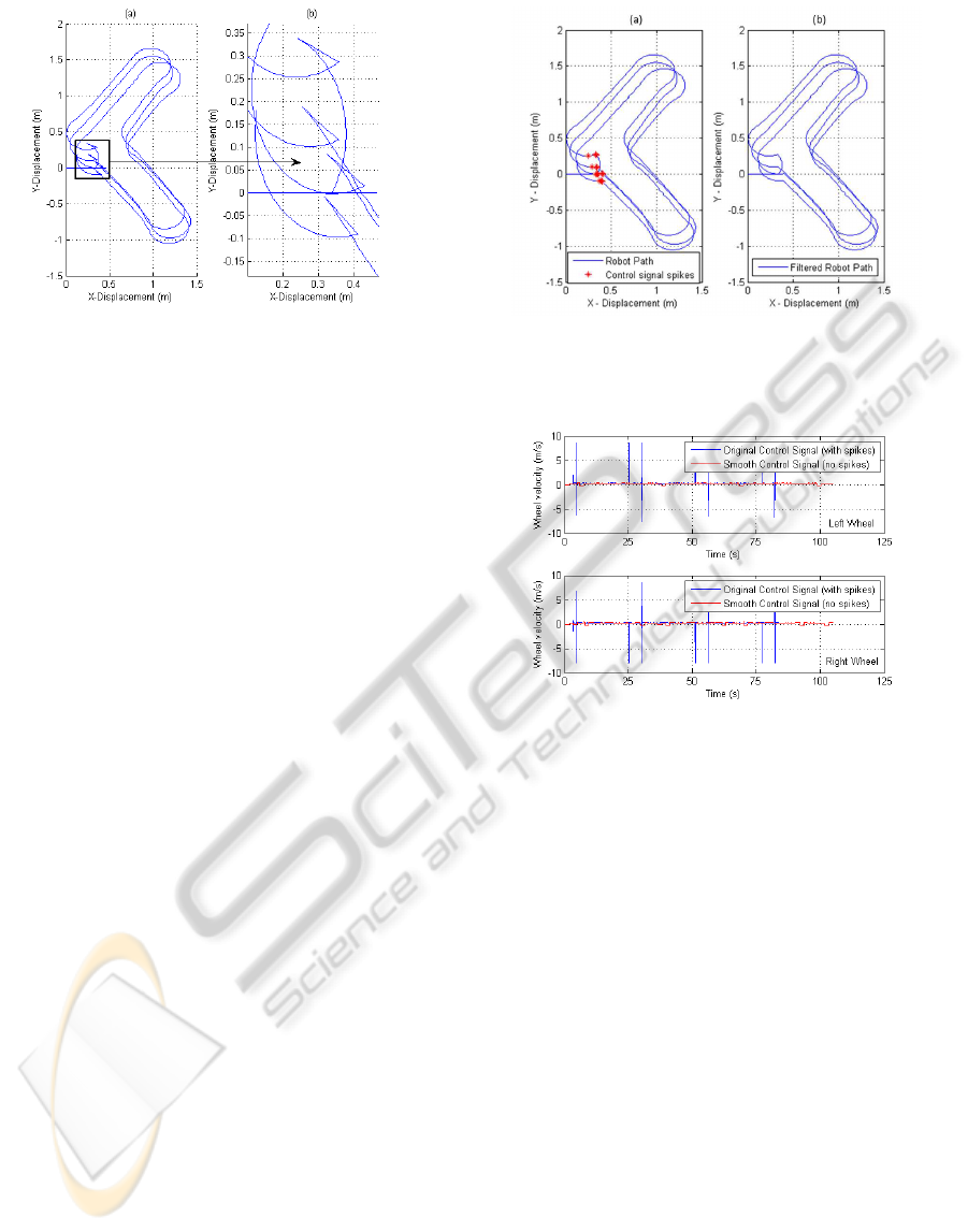
Figure 7: Regions of interest showing ’pinch points’.

to the robot’s exploration route that would result in

the oversight of valuable information. All sections of

’bump and backup’ are therefore classiﬁed as redun-

dant.

Figure 7 shows the regions of interest identiﬁed

based on the mission planner and the correspondingly

computed pinch points. These pinch points are pro-

cessed to delete redundant segments of the path in be-

tween. This task is performed by the redundancy re-

moval module, resulting in a smooth path as shown

in Figure 8 (a). The smooth path is passed as an

input to the re-compute control module which cal-

culates the wheel velocities required to achieve the

new path. The module also notiﬁes the ﬁlter control

signal module of any instantaneous large changes re-

quired in the wheel velocities to help the robot achieve

a speciﬁc position and orientation. These are shown

in Figure 8(a). The ﬁlter control signal module then

interpolates the path as described previously to help

achieve a ﬁnal smoothed path for upload to the main

robot. The processed control signals (before and after

removal of spikes) for each of the wheel modules is

shown in Figure 9. It must be noted that in the newly

calculated path (for upload to the real robot), there

are no collisions with the wall, since this has already

been compensated for from the information provided

by the simulation.

6 EFFECT OF ERRORS IN

PARAMETER ESTIMATION

The mission planning module relies on the estimated

kinematic parameters to determine the robot’s path

in simulation. Speciﬁcally, the module integrates the

wheel velocities over time to determine the path taken

by the robot during the simulated mission. Errors

in the kinematics therefore propagate through all the

modules from an early stage. To illustrate this effect,

Figure 8: (a) Output from the re-compute control module

indicating control signal spikes. (b) Filtered path after re-

moval of control signal spikes by the ﬁnal module.

Figure 9: Control signal (wheel velocities) for the left and

right wheels of the robot.

the estimated wheel base value was modiﬁed by 4%

on either side of the ideal value. The drift in the sim-

ulated path on either side of the actual path as shown

in Figure 10 is a result of this error in the estimate.

The mean squared errors between the actual path and

the resultant error-ridden paths (±4%) are found to be

0.1043 m and 0.1033 m respectively, while the sums

of absolute difference between the paths are found to

be 198.6847 m and 196.7018 m correspondingly.

7 CONCLUSIONS AND FUTURE

WORK

This paper presented a decoupled control paradigm

for the tele-operation of mobile robots. The proposed

control architecture beneﬁts applications that have

to deal with intermittent communication channels or

varying time delays. A general system architecture

has been described that integrates a virtual reality-

based physical simulation and lends itself to rapid

mission planning, modular development and distribu-

GRAPP 2012 - International Conference on Computer Graphics Theory and Applications

560

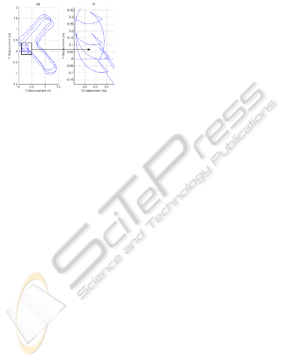
Figure 10: Effect of wrongly estimated wheel base.

tion across a network. Preliminary experimental re-

sults on a sub-section of the control paradigm have

been shown that demonstrate how kinematic parame-

ters of a robot can be estimated and used to improve

simulation results. In addition, an exemplar of a plan-

ning and execution module was described to empha-

size the advantages of the presented system in com-

parison to traditional direct control paradigms.

Since the Augmented Extended Kalman Filter

framework is in place, it can be integrated on the

physical robot to continuously provide an updated

robot state estimate. The presented framework can

accommodate any numbers of sensor inputs, but fus-

ing data from heterogeneous sources is a non-trivial

problem and needs to be investigated. In particular,

how the chosen robot path inﬂuences the evolution

and error covariances of the estimates for the robot’s

kinematic parameters should be investigated.

In addition, the components of the system that

have not been treated here, like environment model-

ing, slave-robot command execution and control need

to be examined and integrated.

REFERENCES

Anykode (2011). anyKode Marilou - Modeling and Simu-

lation Environment for Robotics; Last accessed 2 Jan-

uary 2012.

Arcara, P. and Melchiorri, C. (2002). Control schemes for

teleoperation with time delay : A comparative study.

Robotics and Autonomous Systems, 38:49–64.

Bejczy, A., Kim, W., and Venema, S. (1990). The phantom

robot: predictive displays for teleoperation with time

delay. In Proceedings, IEEE International Conference

on Robotics and Automation, pages 546–551. IEEE

Comput. Soc. Press.

Chong, N. Y., Kotokul, T., Ohba, K., Komoriya, K., Tanie,

K., and Mechanics, E. (2000). Use of Coordinated

On-line Graphics Simulator in Collaborative Multi-

robot Teleoperation with Time Delay. In Proc. IEEE

International Workshop on Robot and Human Inter-

active Communication, pages 167–172, Osaka, Japan.

Hernando, M. and Gambao, E. (2007). Teleprograming:

Capturing the Intention of the Human Operator. In Ad-

vances in Telerobotics, volume 31 of Springer Tracts

in Advanced Robotics, chapter 18, pages 303–320.

Springer.

Hokayem, P. and Spong, M. (2006). Bilateral teleoperation:

An historical survey. Automatica, 42(12):2035–2057.

Jackson, J. (2007). Microsoft robotics studio: A techni-

cal introduction. Robotics & Automation Magazine,

IEEE, 14(4):82–87.

Julier, S. and Uhlmann, J. (2004). Unscented ﬁltering

and nonlinear estimation. Proceedings of the IEEE,

92(3):401–422.

Kalman, R. E. (1960). A New Approach to Linear Filtering

and Prediction Problems. Journal of Basic Engineer-

ing, 82(Series D):35–45.

Kheddar, A. (2001). Teleoperation based on the hidden

robot concept. Systems, Man and Cybernetics, Part A:

Systems and Humans, IEEE Transactions on, 31(1):1–

13.

Kheddar, A., Neo, E., Tadakuma, R., and Yokoi, K.

(2007). Enhanced Teleoperation Through Virtual Re-

ality Techniques. In Ferre, M., Buss, M., Aracil, R.,

Melchiorri, C., and Balaguer, C., editors, Advances

in Telerobotics, volume 31 of Springer Tracts in Ad-

vanced Robotics, chapter 9, pages 139–159. Springer.

Larsen, T. (1998). Optimal Fusion of Sensors. Phd thesis,

Technical University of Denmark.

Martinelli, A., Tomatis, N., and Siegwart, R. (2007). Simul-

taneous localization and odometry self calibration for

mobile robot. Autonomous Robots, 22(1):75–85.

Michel, O. (2004). Webots TM : Professional Mobile

Robot Simulation. International Journal of Advanced

Robotic Systems, 1(1):39–42.

Pan, Y.-j., Canudas-de wit, C., and Sename, O. (2006).

A New Predictive Approach for Bilateral Teleoper-

ation With Applications to Drive-by-Wire Systems.

Robotics, IEEE Transactions on, 22(6):1146–1162.

Wang, C. (1988). Location estimation and uncertainty anal-

ysis for mobile robots. In Proceedings. 1988 IEEE In-

ternational Conference on Robotics and Automation,

pages 1231–1235. IEEE Comput. Soc. Press.

Wright, B. Y. J., Hartman, F., Cooper, B., Maxwell, S.,

Yen, J., and Morrison, J. (2006). Driving on Mars

with RSVP - Building Safe and Effective Command

Sequences. Robotics & Automation Magazine, IEEE,

13(2):37 – 45.

Yu, C.-q., Ju, H.-h., Gao, Y., and Cui, P.-y. (2009). A

Bilateral Teleoperation System for Planetary Rovers.

In 2009 International Conference on Computational

Intelligence and Software Engineering, pages 1–5.

IEEE.

Zhu, J., He, X., and Gueaieb, W. (2011). Trends in

the Control Schemes for Bilateral Teleoperation with

Time Delay. Autonomous and Intelligent Systems,

6752:146–155.

A CONTROL PARADIGM FOR DECOUPLED OPERATION OF MOBILE ROBOTS IN REMOTE ENVIRONMENTS

561