NON-PARAMETRIC SEGMENTATION OF REGIME-SWITCHING

TIME SERIES WITH OBLIQUE SWITCHING TREES

Alexei Bocharov and Bo Thiesson

Microsoft Research, One Microsoft Way, Redmond, WA 98052, U.S.A.

Keywords:

Regime-switching time series, Spectral clustering, Regression tree, Oblique split, Financial markets.

Abstract:

We introduce a non-parametric approach for the segmentation in regime-switching time-series models. The

approach is based on spectral clustering of target-regressor tuples and derives a switching regression tree,

where regime switches are modeled by oblique splits. Our segmentation method is very parsimonious in the

number of splits evaluated during the construction process of the tree–for a candidate node, the method only

proposes one oblique split on regressors and a few targeted splits on time. The regime-switching model can

therefore be learned efﬁciently from data. We use the class of ART time series models to serve as illustration,

but because of the non-parametric nature of our segmentation approach, it readily generalizes to a wide range

of time-series models that go beyond the Gaussian error assumption in ART models. Experimental results on

S&P 1500 ﬁnancial trading data demonstrates dramatically improved predictive accuracy for the exemplifying

ART models.

1 INTRODUCTION

The analysis of time-series data is an important area

of research with applications in areas such as natu-

ral sciences, economics, and ﬁnancial trading to men-

tion a few. Consequently, a wide range of time-series

models and algorithms can be found in the literature.

Many time series exhibit non-stationarity due to

regime switching, and proper detection and modeling

of this switching is a major challenge in time-series

analysis. In regime-switching models, the parame-

ters of the model change between regimes from time

to time in order to reﬂect changes in the underlying

conditions for the time series. As a simple exam-

ple, the volatility or the basic trading value of a stock

may change according to events such as earnings re-

ports or analysts’ upgrades or downgrades. Patterns

may repeat and, as such, it is possible that the model

switches back to a previous regime.

A wide variety of standard mixture modeling ap-

proaches have over the years been adapted to model

regime-switching time series. In Markov-switching

models (see, e.g., Hamilton, 1989, 1990) a Markov

evolving hidden state indirectly partitions the time-

series data to ﬁt local auto-regressive models in the

mixture components. Another large body of work

(see, e.g., Waterhouse and Robinson, 1995; Weigend

et al., 1995) have adapted the hierarchical mixtures

of experts (Jordan and Jacobs, 1994) to regime-

switching time-series models. In these models–also

denoted as gated experts–the hierarchical gates ex-

plicitly operate on the data in order to deﬁne a parti-

tion into local regimes. In both the Markov-switching

and the gated expert models, the determination of the

partition and the local regimes are tightly integrated

in the learning algorithm and demands an iterative ap-

proach, such as the EM algorithm. Furthermore, the

learned partitions have ”soft” boundaries, in the sense

that multiple regimes may contribute to the explana-

tion of data at any point in time.

In this paper, we focus on a more simplistic di-

rection for adapting mixture modeling to regime-

switching time series, which will more easily lend it-

self to explanatory analysis. In that respect, it con-

trasts the above work in the following ways: 1) a

modular separation of the partition and the regime

learning makes it easy to experiment with different

types of models in the local regimes, potentially using

out-of-the-box implementations for the learning, and

2) a direct and deterministic dependence on data in

the switching conditions makes the regime-switching

models easier to interpret.

We model the actual switching conditions in a

regime-switching model in the form of a regression

tree and call it the switching tree. Typically, the con-

struction of a regression tree is a stagewise process

116

Bocharov A. and Thiesson B. (2012).

NON-PARAMETRIC SEGMENTATION OF REGIME-SWITCHING TIME SERIES WITH OBLIQUE SWITCHING TREES.

In Proceedings of the 1st International Conference on Pattern Recognition Applications and Methods, pages 116-125

DOI: 10.5220/0003758601160125

 SciTePress

that involves three ingredients: 1) a split proposer that

creates split candidates to consider for a given (leaf)

node in the tree, 2) one or more scoring criteria for

evaluating the beneﬁt of a split candidate, and 3) a

search strategy that decides which nodes to consider

and which scoring criterion to apply at any state dur-

ing the construction of the tree. Since the seminal

paper (Breiman et al., 1984) popularized the classic

classiﬁcation and regression tree (CART) algorithm,

the research community has given a lot of attention

to both types of decision trees. Many different algo-

rithms have been proposed in the literature by varying

speciﬁcs for the three ingredients in the construction

process mentioned above.

Although there has been much research on learn-

ing regression trees, we know of only one setting,

where these models have been used as switching trees

in regime-switching time series models–namely the

class of auto-regressive tree (ART) models (Meek

et al., 2002). The ART models is a generaliza-

tion of the well-known auto-regressive (AR) mod-

els (e.g.,(Hamilton, 1994)) that is the foundation of

many time-series analyses. The ART models gen-

eralize these models by having a regression tree de-

ﬁne the switching between the different AR models

in the leafs. As such, the well-known threshold auto-

regressive (TAR) models (Tong and Lim, 1980; Tong,

1983) can also be considered as a specialization of an

ART model with the regression tree limited to a sin-

gle split variable. We offer a different approach to

building the switching tree than (Meek et al., 2002),

but we will throughout the paper use the ART models

to both exemplify our approach and at the same time

emphasize the differences with our work.

In particular, we propose a novel improvement to

the way ART creates the candidate splits during the

switching tree construction. A split deﬁnes a predi-

cate, which, given the values of regressor variables,

decides on which side of the split a data case should

belong.

A predicate may be as simple as checking

if the value of a regressor is below some threshold or

not. We will refer to this kind of split as an axial split,

and it is in fact the only type of splits allowed in the

original ART models. Importantly, we show that for a

broad class of time series, the best split is not likely to

be axial, and we therefore extend the switching trees

to allow for so-called oblique splits. The predicate in

an oblique split tests if a linear combination of values

for the regressors is less than a threshold value.

It may sometimes be possible to consider and eval-

uate the efﬁcacy of all feasible axial splits for the

For clarity of presentation, we will focus on binary

splits only. It is a trivial exercise to extend our proposed

method to allow for n-ary splits.

data associated with a node in the tree, but for com-

binatorial reasons, oblique splitting rarely enjoys this

luxury. We therefore need a split proposer, which is

more careful about the candidate splits it proposes. In

fact, our approach is extreme in that respect by only

proposing a single oblique split to be considered for

any given node during the construction of the tree.

Our oblique split proposer involves a simple two step

procedure. In the ﬁrst step, we use a spectral clus-

tering method to separate the data in a node into two

classes. Having separated the data, the second step

now proceeds as a simple classiﬁcation problem, by

using a linear discriminant method to create the best

separating hyperplane for the two data classes. Any

discriminant method can be used, and there is in prin-

ciple no restriction on it being linear, if more compli-

cated splits are sought.

Oblique splitting has enjoyed signiﬁcant attention

for the classiﬁcation tree setting. See, e.g., (Breiman

et al., 1984; Murthy et al., 1994; Brodley and Ut-

goff, 1995; Gama, 1997; Iyengar, 1999). Less atten-

tion has been given to the regression tree setting, but

still a number of methods has come out of the statis-

tics and machine learning communities. See, e.g.,

(Dobra and Gehrke, 2002; Li et al., 2000; Chaud-

huri et al., 1994) to mention a few. Setting aside the

time-series context for our switching trees, the work

in (Dobra and Gehrke, 2002) is in style the most sim-

ilar to the oblique splitting approach that we propose

in this paper. In (Dobra and Gehrke, 2002), the EM

algorithm for Gaussian mixtures is used to cluster the

data. Having committed to Gaussian clusters it now

makes sense to determine a separating hyperplane via

a quadratic discriminant analysis for a projection of

the data onto a vector that ensures maximum separa-

tion of the Gaussians. This vector is found by mini-

mizing Fisher’s separability criterion.

We will in our method do without the dependence

on parametric models when creating an oblique split

candidate for the following two reasons. First of all,

we consider the class of ART models for the pur-

pose of illustration only. Without the dependence

on speciﬁc parametric assumptions, our approach can

be readily generalized to a wide range of time-series

models that go beyond the limit of the Gaussian er-

ror assumption in these models. For example, long-

tailed, skewed, or other non-Gaussian errors, as of-

ten encountered in ﬁnance (see, e.g., Mandelbrot and

Hudson, 2006; Mandelbrot, 1966). Second, it is a

common claim in the literature that spectral cluster-

ing often outperforms traditional parametric cluster-

ing methods, and it has become a popular geometric

clustering tool in many areas of research (see, e.g.,

von Luxburg, 2007).

NON-PARAMETRIC SEGMENTATION OF REGIME-SWITCHING TIME SERIES WITH OBLIQUE SWITCHING

TREES

117

Spectral clustering dates back to the work in (Do-

nath and Hoffman, 1973; Fiedler, 1973) that sug-

gest to use the method for graph partitionings. Vari-

ations of spectral clustering have later been popu-

larized in the machine learning community (Shi and

Malik, 2000; Meil

a and Shi, 2001; Ng et al., 2002),

and, importantly, very good progress has been made

in improving an otherwise computationally expensive

eigenvector computation for these methods (White

and Smyth, 2005). We use a simple variation of the

method in (Ng et al., 2002) to create a spectral clus-

tering for the time series data in a node. Given this

clustering, we then use a simple perceptron learning

algorithm (e.g., (Bishop, 1995)) to ﬁnd a hyperplane

that deﬁnes a good oblique split predicate for the au-

toregressors in the model.

Let us now turn to the possibility of splitting on

the time feature in a time series. Due to the special

nature of time, it does not make sense to involve this

feature as an extra dimension in the spectral cluster-

ing; it would not add any discriminating power to the

method. Instead, we propose a procedure for time

splits, which uses the spectral clustering in another

way. The procedure identiﬁes speciﬁc points in time,

where succeeding data elements in the series cross the

cluster boundary, and proposes time splits at those

points. Our split proposer will in this way use the

spectral clustering to produce both the oblique split

candidate for the regressors, and a few very targeted

(axial) split candidates for the time dimension.

The rest of the paper is organized as follows. In

Section 2, we brieﬂy review the ART models that

we use to exemplify our work, and we deﬁne and

motivate the extension that allows for oblique splits.

Section 3 reviews the general learning framework for

ART models. Section 4 contains the details for both

aspects of our proposed spectral splitting method–

the oblique splitting and the time splitting. In Sec-

tions 5 and 6 we describe experiments and provide ex-

perimental evidence demonstrating that our proposed

spectral splitting method dramatically improves the

quality of the learned ART models over the current

approach. We will conclude in Section 7.

2 STANDARD AND OBLIQUE

ART MODELS

We begin by introducing some notation. We de-

note a temporal sequence of variables by X =

,...,X

), and we denote a sub-sequence con-

sisting of the i’th through the j’th element by X

i+1

,...,X

), i < j. Time-series data is a se-

quence of values for these variables denoted by x =

,...,x

). We assume continuous values, ob-

tained at discrete, equispaced intervals of time.

An autoregressive (AR) model of length p, is sim-

ply a p-order Markov model that imposes a linear re-

gression for the current value of the time series given

the immediate past of p previous values. That is,

p(x

t−1

) = p(x

t−1

t−p

) ∼ N (m +

∑

j=1

t−j

,σ

)

where N (µ,σ

) is a conditional normal distri-

bution with mean µ and variance σ

, and θ =

(m,b

,...,b

,σ

) are the model parameters (?,

e.g.,)page 55]DeGroot:1970.

The ART models is a regime-switching general-

ization of the AR models, where a switching regres-

sion tree determines which AR model to apply at each

time step. The autoregressors therefore have two pur-

poses: as input for a classiﬁcation that determines a

particular regime, and as predictor variables in the

linear regression for the speciﬁc AR model in that

regime.

As a second generalization

, ART models may al-

low exogenous variables, such as past observations

from related time series, as regressors in the model.

Time (or time-step) is a special exogenous variable,

only allowed in a split condition, and is therefore only

used for modeling change points in the series.

2.1 Axial and Oblique Splits

Different types of switching regression trees can be

characterized by the kind of predicates they allow for

splits in the tree. The ART models allow only a simple

form of binary splits, where a predicate tests the value

of a single regressor. The models handle continuous

variables, and a split predicate is therefore of the form

≤ c

where c is a constant value and X

is any one of the re-

gressors in the model or a variable representing time.

A simple split of this type is also called axial, because

the predicate that splits the data at a node can be con-

sidered as a hyperplane that is orthogonal to the axis

for one of the regressor variables or the time variable.

The best split for a node in the tree can be learned

by considering all possible partitionings of the data

according to each of the individual regressors in the

model, and then picking the highest scoring split for

these candidates according to some criterion. It can,

The class of ART models with exogenous variables has

not been documented in any paper. We have learned about

this generalization from communications with the authors

of (Meek et al., 2002).

ICPRAM 2012 - International Conference on Pattern Recognition Applications and Methods

118

however, be computationally demanding to evaluate

scores for that many split candidates, and for that rea-

son, (Chickering et al., 2001) investigated a Gaussian

quantile approach that proposes only 15 split points

for each regressor. They found that this approach

is competitive to the more exhaustive approach. A

commercial implementation for ART models uses the

Gaussian quantile approach and we will compare our

alternative to this approach.

We propose a solution, which will only produce

a single split candidate to be considered for the en-

tire set of regressors. In this solution we extend the

class of ART models to allow for a more general split

predicate of the form

∑

≤ c (1)

where the sum is over all the regressors in the model

and a

are corresponding coefﬁcients. Splits of this

type are in (Murthy et al., 1994) called oblique due to

the fact that a hyperplane that splits data according to

the linear predicate is oblique with respect to the re-

gressor axes. We will in Section 4 describe the details

behind the method that we use to produce an oblique

split candidate.

2.2 Motivation for Oblique Splits

There are general statistical reasons why, in many sit-

uations, oblique splits are preferable over axial splits.

In fact, for a broad class of time series, the best

splitting hyperplane turns out to be approximately or-

thogonal to the principal diagonal d = (

√

,...,

√

To qualify this fact, consider two pre-deﬁned classes

of segments x

(c)

,c = 1, 2 for the time-series data x.

Let µ

(c)

and Σ

(c)

denote the mean vector and covari-

ance matrix for the sample joint distribution of X

t−1

t−p

computed for observations on p regressors for targets

∈ x

(c)

Let us deﬁne the moving average A

∑

i=1

t−i

We show in the Appendix that in the context where

t−i

−A

is weakly correlated with A

, while its vari-

ance is comparable with that of A

, the angle between

the principal diagonal and one of the principal axes

of Σ

(c)

,c = 1,2 is small. This would certainly be the

case with a broad range of ﬁnancial data, where in-

crements in price curves have notoriously low corre-

lations with price values (Samuelson, 1965; Mandel-

brot, 1966), while seldom overwhelming the averages

in magnitude. With one of the principal axes being

approximately aligned with the principal diagonal d

for both Σ

(1)

and Σ

(2)

it is unlikely that a cut orthogo-

nal to either of the coordinate axes X

t−1

,...,X

t−p

can

provide optimal separation of the two classes. (The

argument depends on all eigenvalues for Σ

(c)

being

distinct; a somewhat different argument involving the

geometry of mean vectors µ

(c)

is needed in the special

case, where the eigenvalues are not distinct.)

3 THE LEARNING PROCEDURE

An ART model is typically learned in a stagewise

fashion. The learning process starts from the trivial

model without any regressors and then greedily adds

regressors one at a time until the learned model does

not improve a chosen scoring criterion. The candi-

date regressors considered at any given stage in this

process consist of the autoregressor one step further

back in time than currently accepted in the model and

possibly a preselected set of exogenous variables from

related cross-predicting time series.

The task of learning a speciﬁc autoregressive

model considered at any stage in this process can be

cast into a standard task of learning a linear regres-

sion tree. It is done by a trivial transformation of

the time-series data into multivariate data cases for

the regressor and target variables in the model. For

example, when learning an ART model of length p

with an exogenous regressor, say z

t−q

, from a re-

lated time series, the transformation creates the set of

T − max(p, q) cases of the type (x

t−p

t−q

), where

max(p,q) + 1 < t ≤ T . We will in the following de-

note this transformation as the phase view, due to a

vague analogy to the phase trajectory in the theory of

dynamical systems.

Most regression tree learning algorithms construct

a tree in two stages (see, e.g., Breiman et al., 1984):

First, in a growing stage, the learning algorithm will

maximize a scoring criterion by recursively trying to

replace leaf nodes by better scoring splits. A least-

squares deviation criterion is often used for scoring

splits in a regression tree. Typically the chosen crite-

rion will cause the selection of an overly large tree

with poor generalization. In a pruning stage, the

tree is therefore pruned back by greedily eliminating

leaves using a second criterion–such as the holdout

score on a validation data set–with the goal of mini-

mizing the error on unseen data.

In contrast, (Meek et al., 2002) suggests a learn-

ing algorithm that uses a Bayesian scoring criterion,

described in detail in that paper. This criterion avoids

over-ﬁtting by penalizing for the complexity of the

model, and consequently, the pruning stage is not

needed. We use this Bayesian criterion in our experi-

mental section.

In the next section, we describe the details of the

algorithm we propose for producing the candidate

NON-PARAMETRIC SEGMENTATION OF REGIME-SWITCHING TIME SERIES WITH OBLIQUE SWITCHING

TREES

119

splits that are considered during the recursive con-

struction of a regression tree. Going from axial to

oblique splits adds complexity to the proposal of can-

didate splits. However, our split proposer dramati-

cally reduces the number of proposed split candidates

for the nodes evaluated during the construction of the

tree, and by virtue of that fact spends much less time

evaluating scores of the candidates.

4 SPECTRAL SPLITTING

This section will start with a brief description of spec-

tral clustering, followed by details about how we ap-

ply this method to produce candidate splits for an

ART time-series model. A good tutorial treatment

and an extensive list of references for spectral clus-

tering can be found in (von Luxburg, 2007).

The spectral splitting method that we propose

constructs two types of split candidates–oblique and

time–both relying on spectral clustering. Based on

this clustering, the method applies two different views

on the data–phase and trace–according to the type of

splits we want to accomplish. The algorithm will only

propose a single oblique split candidate and possibly a

few time split candidates for any node evaluated dur-

ing the construction of the regression tree.

4.1 Spectral Clustering

Given a set of n multi-dimensional data points

,...,x

), we let a

i j

= a(x

) denote the afﬁn-

ity between the i’th and j’th data point, accord-

ing to some symmetric and non-negative measure.

The corresponding afﬁnity matrix is denoted byA =

i j

)

i, j=1,...,n

, and we let D denote the diagonal matrix

with values

∑

j=1

i j

, i = 1,...,n on the diagonal.

Spectral clustering is a non-parametric clustering

method that uses the pairwise afﬁnities between data

points to formulate a criterion that the clustering must

optimize. The trick in spectral clustering is to en-

hance the cluster properties in the data by changing

the representation of the multi-dimensional data into

a (possibly one-dimensional) representation based on

eigenvalues for the so-called Laplacian.

L = D −A

Two different normalizations for the Laplacian have

been proposed in (Shi and Malik, 2000) and (Ng et al.,

2002), leading to two slightly different spectral clus-

tering algorithms. We will follow a simpliﬁed version

of the latter. Let I denote the identity matrix. We

will cluster the data according to the second small-

est eigenvector–the so-called Fiedler vector (Fiedler,

1973)–of the normalized Laplacian

norm

= D

−1/2

= I −D

−1/2

The algorithm is illustrated in Figure 1. Notice that

we replace L

norm

with

norm

= I −L

norm

which changes eigenvalues from λ

to 1 − λ

and

leaves eigenvectors unchanged. We therefore ﬁnd the

eigenvector for the second-largest and not the second-

smallest eigenvector. We prefer this interpretation of

the algorithm for reasons that become clear when we

discuss iterative methods for ﬁnding eigenvalues in

Section 4.2.

1. Construct the matrix L

norm

2. Find the second-largest eigenvector e =

,...,e

) of L

norm

3. Cluster the elements in the eigenvector (e.g.

by the largest gap in values).

4. Assign the original data point x

to the clus-

ter assigned to e

Figure 1: Simple normalized spectral clustering algorithm.

Readers familiar with the original algorithm in

(Ng et al., 2002) may notice the following simpliﬁ-

cations: First, we only consider a binary clustering

problem, and second, we only use the two largest

eigenvectors for the clustering, and not the k largest

eigenvectors in their algorithm. (The elements in the

ﬁrst eigenvector always have the same value and will

therefore not contribute to the clustering.) Due to

the second simpliﬁcation, the step in their algorithm

that normalizes rows of stacked eigenvectors can be

avoided, because the constant nature of the ﬁrst eigen-

vector leaves the transformation of the second eigen-

vector monotone.

4.2 Oblique Splits

Oblique splits are based on a particular view of the

time series data that we call the phase view, as de-

ﬁned in Section 3. Importantly, a data case in the

phase view involves values for both the target and re-

gressors, which imply that our oblique split proposals

may capture regression structures that show up in the

data–as opposed to many standard methods for axial

splits that are ignorant to the target when determining

split candidates for the regressors.

It should also be noted that because the phase view

has no notion of time, similar patterns from entirely

different segments of time may end up on the same

side of an oblique split. This property can at times

ICPRAM 2012 - International Conference on Pattern Recognition Applications and Methods

120

result in a great advantage over splitting the time se-

ries into chronological segments. First of all, splitting

on time imposes a severe constraint on predictions,

because splits in time restrict the prediction model to

information from the segment latest in time. Informa-

tion from similar segments earlier in the time series

are not integrated into the prediction model in this

case. Second, we may need multiple time splits to

mimic the segments of one oblique split, which may

not be obtainable due to the degradation of the statis-

tical power from the smaller segments of data. Fig-

ure 2(d) shows an example, where a single oblique

split separates the regime with the less upward trend-

ing and slightly more volatile ﬁrst and third data seg-

ments of the time series from the regime consisting of

the less volatile and more upward trending second and

fourth segments. In contrast, we would have needed

three time splits to properly divide the segments and

these splits would therefore have resulted in four dif-

ferent regimes.

Our split proposer produces a single oblique split

candidate in a two step procedure. In the ﬁrst step, we

strive to separate two modes that relates the target and

regressors for the model in the best possible way. To

accomplish this task, we apply the afﬁnity based spec-

tral clustering algorithm, described in Section 4.1, to

the phase view of the time series data. For the exper-

iments reported later in this paper, we use an afﬁnity

measure proportional to

1 + ||p

−p

where ||p

− p

is the L2-norm between two

phases. We do not consider exogenous regressors

from related time series in these experiments. All

variables in the phase view are therefore on the same

scale, making the inverse distance a good measure

of proximity. With exogenous regressors, more care

should be taken with respect to the scaling of variables

in the proximity measure, or the time series should be

standardized. Figure 2(b) demonstrates the spectral

clustering for the phase view of the time-series data

in Figure 2(a), where this phase view has been con-

structed for an ART model with two autoregressors.

The oblique split predicate in (1) deﬁnes an in-

equality that only involves the regressors in the

model. The second step of the oblique split pro-

poser therefore projects the clustering of the phase

view data to the space of the regressors, where the

hyperplane separating the clusters is now constructed.

While this can be done with a variety of linear dis-

crimination methods, we decided to use a simple

single-layer perceptron optimizing the total misclas-

siﬁcation count. Such perceptron will be relatively

insensitive to outliers, compared to, for example,

Fisher’s linear discriminant.

The computational complexity of an oblique split

proposal is dominated by the cost of computing the

full afﬁnity matrix, the second largest eigenvector for

the normalized Laplacian, and ﬁnding the separating

hyperplane for the spectral clusters. Recall that n de-

notes the number of cases in the phase view of the

data. The cost of computing the full afﬁnity matrix is

therefore O(n

) afﬁnity computations. Direct meth-

ods for computing the second largest eigenvector is

O(n

). A complexity of O(n

) may be prohibitive

for series of substantial length. Fortunately, there are

approximate iterative methods, which in practice are

much faster with tolerant error. For example, the Im-

plicitly Restarted Lanczos Method (IRLM) has com-

plexity O(mh + nh), where m is the number of non-

zero afﬁnities in the afﬁnity matrix and h is the num-

ber of iterations required until convergence (White

and Smyth, 2005). With a full afﬁnity matrix m = n

but a signiﬁcant speedup can be accomplished by only

recording afﬁnities above a certain threshold in the

afﬁnity matrix. Finally, the perceptron algorithm has

complexity O(nh).

4.3 Time Splits

A simple but computationally expensive way of de-

termining a good time split is to let the split pro-

poser nominate all possible splits in time for the fur-

ther evaluation. The commercial implementation of

the ART models relies on an approximation to this

approach that proposes a smaller set of equispaced

points on the time axis.

We suggest a data driven approximation, which

will more precisely target the change points in the

time series. Our approach is based on another view

of the time series data that we call the trace view. In

the trace view we use the additional time information

to label the phase view data in the spectral clustering.

The trace view, now traces the clustered data through

time and proposes a split point each time the trace

jumps across clusters. The rationale behind our ap-

proach is that data in the same cluster will behave in a

similar way, and we can therefore signiﬁcantly reduce

the number of time-split proposals by only proposing

the cluster jumps. As an example, the thin lines or-

thogonal to the time axis in Figure 2(d) shows the few

time splits proposed by our approach. Getting close

to a good approximation for the equispaced approach

would have demanded far more proposed split points.

Turning now to the computational complexity.

Assuming that spectral clustering has already been

performed for the oblique split proposal, the addi-

tional overhead for the trace through data is O(n).

NON-PARAMETRIC SEGMENTATION OF REGIME-SWITCHING TIME SERIES WITH OBLIQUE SWITCHING

TREES

121

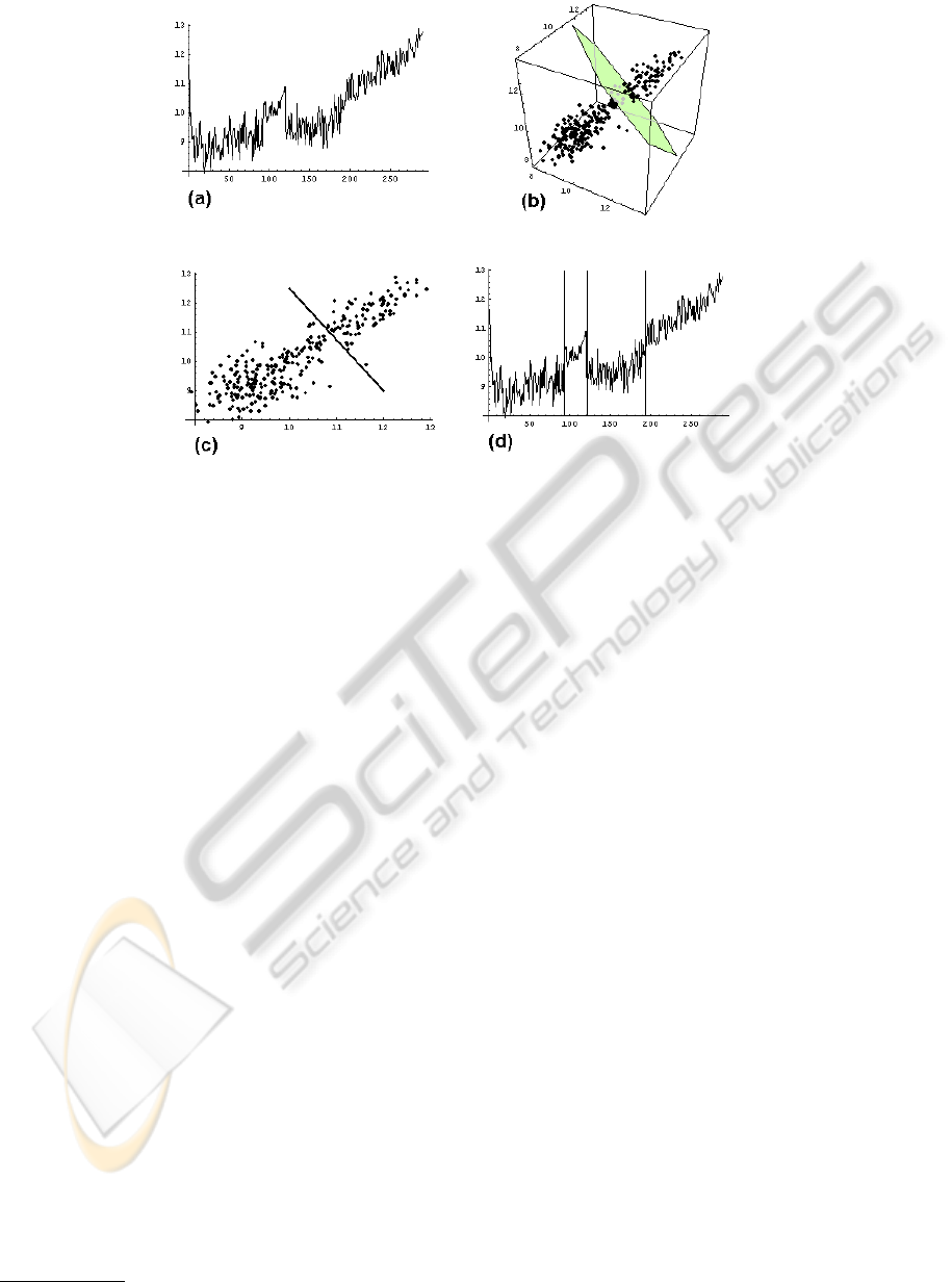
Figure 2: Oblique split candidate for ART model with two autoregressors. (a) The original time series. (b) The spectral

clustering of phase-view data. The polygon separating the upper and lower parts is a segment of a separating hyperplane for

the spectral clusters (c) The phase view projection to regressor plane and the separating hyperplane learned by the perceptron

algorithm. (d) The effect of the oblique split on the original time series: a regime consisting of the slightly less upward

trending and more volatile ﬁrst and third data segments is separated from the regime with more upward trending and less

volatile second and fourth segments.

5 EVALUATION

In this section, we provide an empirical evaluation for

our spectral splitting methods. We use a large collec-

tion of ﬁnancial trading data. The collection contains

the daily closing prices for 1495 stocks from Standard

& Poor’s 1500 index

as of January 1, 2008. Each

time series spans across approximately 150 trading

days ending on February 1, 2008. (Rotation of stocks

in the S&P 1500 lead to the exclusion of 5 stocks with

insufﬁent data.) The historic price data is available

from Yahoo!, and can be downloaded with queries of

format http://ﬁnance.yahoo.com/q/hp?s=SYMBOL,

where SYMBOL is the symbol for the stock in the

index. We divide each data set into a training set,

used as input to the learning method, and a holdout

set, used to evaluate the models. We use the last ﬁve

observations as the holdout set, knowing that the data

are daily with trading weeks of ﬁve days.

In our experiments, we learn ART models with an

arbitrary number of autoregressors and we allow time

as an exogenous split variable. We do not complicate

the experiments with the use of exogenous regressors

from related time series, as this complication is irrele-

vant to the objective for this paper. For all the models

that we learn, we use the same Bayesian scoring cri-

standardandpoors.com

terion, the same greedy search strategy for ﬁnding the

number of autoregressors, and the same method for

constructing a regression tree – except that different

alternative split candidates are considered for the dif-

ferent splitting algorithms that we consider.

We evaluate two different types of splitting with

respect to the autoregressors in the model: Axial-

Gaussian and ObliqueSpectral. The AxialGaussian

method is the standard method used to propose mul-

tiple axial candidates for each split in an ART model,

as described in Section 2.1. The ObliqueSpectral

method is our proposed method, which for a split con-

siders only a single oblique candidate involving all re-

gressors. In combination with the two split proposer

methods for autoregressors, we also evaluate three

types of time splitting: NoSplit, Fixed, and Time-

Spectral. The NoSplit method does not allow any

time splits. The Fixed method is the simple standard

method for learning splits on time in an ART model,

as described in Section 4.3. The TimeSpectral method

is our spectral clustering-based alternative. In order

to provide context for the numbers in the evaluation

of these methods, we will also evaluate a very weak

baseline, namely the method not allowing any splits.

We call this method the Baseline method.

We evaluate the quality of a learned model by

computing the sequential predictive score for the

ICPRAM 2012 - International Conference on Pattern Recognition Applications and Methods

122

holdout data set corresponding to the training data

from which the model was learned. The sequential

predictive score for a model is simply the average log-

likelihood obtained by a one-step forecast for each of

the observations in the holdout set. To evaluate the

quality of a learning method, we compute the average

of the sequential predictive scores obtained for each

of the time series in the collection. Note that the use

of the log-likelihood to measure performance simul-

taneously evaluates both the accuracy of the estimate

and the accuracy of the uncertainty of the estimate.

Finally, we use a (one-sided) sign test to evaluate if

one method is signiﬁcantly better than another. To

form the sign test, we count the number of times one

method improves the predictive score over the other

for each individual time series in the collection. Ex-

cluding ties, we seek to reject the hypothesis of equal-

ity, where the test statistic for the sign test follows a

binomial distribution with probability parameter 0.5.

6 RESULTS

To make sure that the results reported here are not

an artifact of sub-optimal axial splitting for the Ax-

ialGaussian method, we ﬁrst veriﬁed the claim from

(Chickering et al., 2001) that the Gaussian quantiles

is a sufﬁcient substitute for the exhaustive set of pos-

sible axial splits. We compared the sequential predic-

tive scores on 10% of the time series in our collection

and did not ﬁnd a signiﬁcant difference.

Table 1 shows the average sequential predictive

scores across the series in our collection for each

combination of autoregressor and time-split proposer

methods. First of all, for splits on autoregressors, we

see a large improvement in score with our Oblique-

Spectral method over the standard AxialGaussian

method. Even with the weak baseline–namely the

method not allowing any splits–the relative improve-

ment from AxialGaussian to ObliqueSpectral over the

improvement from the baseline to AxialGaussian is

still above 20%, which is quite impressive.

The fractions in Table 2 report the number of times

one method has higher score than another method for

all the time series in our collection. Notice that the

numbers in a fraction do not necessarily sum to 1495,

because we are not counting ties. We particularly no-

tice that the ObliqueSpectral method is signiﬁcantly

better than the standard AxialGaussian method for all

three combinations with time-split proposer methods.

In fact, the sign test rejects the hypothesis of equality

at a signiﬁcance level < 10

−5

in all cases. Combin-

ing the results from Tables 1 and 2, we can conclude

that the large improvement in the sequential predic-

Table 1: Average sequential predictive scores for each com-

bination of autoregressor and time split proposer methods.

Regressor splits Time splits Ave. score

Baseline Baseline -3.07

AxialGaussian NoSplit -1.73

AxialGaussian Fixed -1.72

AxialGaussian TimeSpectral -1.74

ObliqueSpectral NoSplit -1.45

ObliqueSpectral Fixed -1.46

ObliqueSpectral TimeSpectral -1.44

Table 2: Pairwise comparisons of sequential predictive

scores. The fractions show the number of time series, where

one method has higher score than the other. The column

labels denote the autoregressor split proposers being com-

pared.

Baseline / Baseline / AxialGaussian /

AxialGaussian ObliqueSpectral ObliqueSpectral

NoSplit 118 / 959 74 / 1168 462 / 615

Fixed 114 / 990 79 / 1182 226 / 418

SpectralTime 122 / 955 71 / 1171 473 / 604

tive scores for our ObliqueSpectral method over the

standard AxialGaussian method is due to a general

trend in scores across individual time series, and not

just a few outliers.

We now turn to the surprising observation that

adding time-split proposals to either of the Axial-

Gaussian and the ObliqueSpectral autoregressor pro-

posals does not improve the quality over models

learned without time splits–neither for the Fixed nor

the TimeSpectral method. Apparently, the axial and

oblique splitting on autoregressors are ﬂexible enough

to cover the time splits in our analysis. We do not

necessarily expect this ﬁnding to generalize beyond

series that behave like stock data, due to the fact that

it is a relatively easy exercise to construct an artiﬁcial

example that will challenge this ﬁnding.

Finally, the oblique splits proposed by our method

involve all regressors in a model, and therefore rely

on our spectral splitting method to be smart enough to

ignore noise that might be introduced by irrelevant re-

gressors. Although efﬁcient, such parsimonious split

proposal may appear overly restrictive compared to

the possibility of proposing split candidates for all

possible subsets of regressors. However, an additional

set of experiments have shown that the exhaustive ap-

proach in general only leads to insigniﬁcant improve-

ments in predictive scores. We conjecture that the

NON-PARAMETRIC SEGMENTATION OF REGIME-SWITCHING TIME SERIES WITH OBLIQUE SWITCHING

TREES

123

stagewise inclusion of regressors in the overall learn-

ing procedure for an ART model (see Section 3) is a

main reason for irrelevant regressors to not pose much

of a problem for our approach.

7 CONCLUSIONS AND FUTURE

WORK

We have presented a spectral splitting method that

improves segmentation in regime-switching time se-

ries, and use the segmentation in the process of cre-

ating a switching regression tree for the regimes in

the model. We have exempliﬁed our approach by

an extension to the ART models–the only type of

models that to our knowledge applies switching trees

in regime-switching models. However, the spectral

splitting method does not rely on speciﬁc paramet-

ric assumptions, which allows for our approach to

be readily generalized to a wide range of regime-

switching time-series models that go beyond the limit

of the Gaussian error assumption in the ART mod-

els. Our proposed method is very parsimonious in

the number of split predicates it proposes for candi-

date split nodes in the tree. It only proposes a single

oblique split candidate for the regressors in the model

and possibly a few very targeted time-split candidates,

thus keeping computational complexity of the over-

all algorithm under control. Both types of split can-

didates rely on a spectral clustering, where different

views–phase and trace–on the time-series data give

rise to the two different types of candidates.

Finally, we have given experimental evidence that

our approach, when applied for the exemplifying ART

models, dramatically improves predictive accuracy

over the current approach. Regarding time splits,

we hope to be able to ﬁnd–and are actively looking

for–real-world time series for future experiments that

will allow us to factor out and compare the quality of

our spectral time-split proposer method to the current

ART approach.

The focus in this paper has been on learning

regime-switching time-series models that will easily

lend themselves to explanatory analysis and interpre-

tation. In future experiments we also plan to evaluate

the potential tradeoff in modularity, interpretability,

and computational efﬁciency with forecast precision

for our simple learning approach compared to more

complicated approaches that integrates learning of

soft regime switching and the local regimes the mod-

els, such as the learning of Markov-switching (e.g.

Hamilton, 1989, 1990) and gated expert (e.g. Wa-

terhouse and Robinson, 1995; Weigend et al., 1995)

models.

REFERENCES

Bishop, C. M. (1995). Neural Networks for Pattern Recog-

nition. Oxford University Press, Oxford.

Breiman, L., Friedman, J. H., Olshen, R. A., and Stone,

C. J. (1984). Classiﬁcation and Regression Trees.

Wadsworth International Group, Belmont, California.

Brodley, C. E. and Utgoff, P. E. (1995). Multivariate deci-

sion trees. Machine Learning, 19(1):45–77.

Chaudhuri, P., Huang, M. C., Loh, W.-Y., and Yao, R.

(1994). Piecewise polynomial regression trees. Sta-

tistica Sinica, 4:143–167.

Chickering, D., Meek, C., and Rounthwaite, R. (2001).

Efﬁcient determination of dynamic split points in a

decision tree. In Proc. of the 2001 IEEE Inter-

national Conference on Data Mining, pages 91–98.

IEEE Computer Society.

DeGroot, M. (1970). Optimal Statistical Decisions.

McGraw-Hill, New York.

Dobra, A. and Gehrke, J. (2002). Secret: A scalable lin-

ear regression tree algorithm. In Proc. of the 8th

ACM SIGKDD International Conference on Knowl-

edge Discovery and Data Mining, pages 481–487.

ACM Press.

Donath, W. E. and Hoffman, A. J. (1973). Lower bounds for

the partitioning of graphs. IBM Journal of Research

and Development, 17:420–425.

Fiedler, M. (1973). Algebraic connectivity of graphs.

Czechoslovak Mathematical Journal, 23:298–305.

Gama, J. (1997). Oblique linear tree. In Proc. of the Second

International Symposium on Intelligent Data Analy-

sis, pages 187–198.

Hamilton, J. (1994). Time Series Analysis. Princeton Uni-

versity Press, Princeton, New Jersey.

Hamilton, J. D. (1989). A new approach to the economic

analysis of nonstationary time series and the business

cycle. Econometrica, 57(2):357–84.

Hamilton, J. D. (1990). Analysis of time series subject to

changes in regime. Journal of Econometrics, 45:39–

70.

Iyengar, V. S. (1999). Hot: Heuristics for oblique trees. In

Proc. of the 11th IEEE International Conference on

Tools with Artiﬁcial Intelligence, pages 91–98, Wash-

ington, DC. IEEE Computer Society.

Jordan, M. I. and Jacobs, R. A. (1994). Hierarchical mix-

tures of experts and the EM algorithm. Neural Com-

putation, 6:181–214.

Li, K. C., Lue, H. H., and Chen, C. H. (2000). Interactive

tree-structured regression via principal Hessian direc-

tions. Journal of the American Statistical Association,

95:547–560.

Mandelbrot, B. (1966). Forecasts of future prices, unbiased

markets, and martingale models. Journal of Business,

39:242–255.

Mandelbrot, B. B. and Hudson, R. L. (2006). The

(mis)Behavior of Markets: A Fractal View of Risk,

Ruin And Reward. Perseus Books Group, New York.

Meek, C., Chickering, D. M., and Heckerman, D. (2002).

Autoregressive tree models for time-series analysis. In

Proc. of the Second International SIAM Conference

on Data Mining, pages 229–244. SIAM.

ICPRAM 2012 - International Conference on Pattern Recognition Applications and Methods

124

Meil

a, M. and Shi, J. (2001). Learning segmentation by ran-

dom walks. In Advances in Neural Information Pro-

cessing Systems 13, pages 873–879. MIT Press.

Murthy, S. K., Kasif, S., and Salzberg, S. (1994). A sys-

tem for induction of oblique decision trees. Journal of

Artiﬁcial Intelligence Research, 2:1–32.

Ng, A. Y., Jordan, M. I., and Weiss, Y. (2002). On spectral

clustering: Analysis and an algorithm. In Advances

in Neural Information Processing Systems 14, pages

849–856. MIT Press.

Samuelson, P. (1965). Proof that properly anticipated prices

ﬂuctuate randomly. In Industrial Management Re-

view, volume 6, pages 41–49.

Shi, J. and Malik, J. (2000). Normalized cuts and image

segmentation. IEEE Transactions on Pattern Analysis

and Machine Intelligence, 22(8):888–905.

Tong, H. (1983). Threshold models in non-linear time se-

ries analysis. In Lecture notes in statistics, No. 21.

Springer-Verlag.

Tong, H. and Lim, K. S. (1980). Threshold autoregres-

sion, limit cycles and cyclical data- with discussion.

Journal of the Royal Statistical Society, Series B,

42(3):245–292.

von Luxburg, U. (2007). A tutorial on spectral clustering.

Statistics and Computing, 17(4):395–416.

Waterhouse, S. and Robinson, A. (1995). Non-linear pre-

diction of acoustic vectors using hierarchical mixtures

of experts. In Advances in Neural Information Pro-

cessing Systems 7, pages 835–842. MIT Press.

Weigend, A. S., Mangeas, M., and Srivastava, A. N. (1995).

Nonlinear gated experts for time series: Discovering

regimes and avoiding overﬁtting. International Jour-

nal of Neural Systems, 6(4):373–399.

White, S. and Smyth, P. (2005). A spectral clustering ap-

proach to ﬁnding communities in graphs. In Proc. of

the 5th SIAM International Conference on Data Min-

ing. SIAM.

APPENDIX

Lemma 1. Let Σ be a non-singular sample auto-

covariance matrix for X

t−1

t−p

deﬁned on the p-

dimensional space with principal diagonal direction

d = (

√

,...,

√

), and let A

∑

i=1

t−i

. Then

sin

(Σd,d) =

∑

i=1

cov(X

t−i

−A

)

∑

i=1

cov(X

t−i

)

. (2)

Proof. Introduce S

∑

i=1

t−i

. As per bi-linear

property of covariance, (Σd)

√

cov(X

t−i

),i =

1,..., p and (Σd)d =

∑

i=1

cov(X

t−i

) =

cov(A

). Non-singularity of Σ implies that

the vector Σd 6= 0. Hence, |Σd|

6= 0 and

cos

(Σd,d) =

((Σd)d)

|(Σd)|

p cov(A

)

∑

i=1

cov(X

t−i

)

It follows that

sin

(Σd,d)

= 1 −cos

(Σd,d)



∑

i=1

cov(X

t−i

)

−cov(A

)



∑

i=1

cov(X

t−i

)

∑

i=1

cov(X

t−i

−A

)

∑

i=1

cov(X

t−i

)

Dividing the numerator and denominator of the last

fraction by p

amounts to replacing S

by A

, which

concludes the proof. 2

Corollary 1. When X

t−i

−A

and A

are weakly cor-

related, and the variance of X

t−i

−A

is comparable

to that of A

, i = 1,..., p, then sin

(Σd,d) is small.

Speciﬁcally, let σ and ρ denote respectively stan-

dard deviation and correlation, and introduce ∆

cov(X

t−i

−A

)

σ(A

)

= ρ(X

t−i

− A

)σ(X

t−i

− A

). We

quantify both assumptions in Corollary 1 by positing

that |∆

|< εσ(A

),i = 1,..., p, where 0 < ε 1. Easy

algebra on Equation (2) yields

sin

(Σd,d) =

Σ∆

Σ(σ(A

) + ∆

)

pε

σ(A

)

p(1 −ε)

σ(A

)

(1 −ε)

(3)

Under the assumptions of Corollary 1, we can now

show that d is geometrically close to an eigenvector of

Σ. Indeed, by inserting (3) into the Pythagorean iden-

tity we derive that |cos(Σd,d)| >

√

1−2ε

1−ε

and close to

1. Now, given a vector v for which |v|= 1, |cos(Σv,v)|

reaches the maximum of 1 iff v is an eigenvector of Σ.

When the eigenvalues of Σ are distinct, d must there-

fore be at a small angle with one of the p principal

axes for Σ.

NON-PARAMETRIC SEGMENTATION OF REGIME-SWITCHING TIME SERIES WITH OBLIQUE SWITCHING

TREES

125