
Network Monitoring and Personalized Traffic Control: A
Starting Point based on Experiences from the
Municipality of Enschede in the Netherlands
Tom Thomas and Sander Veenstra
Center of Transport Studies, University of Twente, P.o box 217
7500 AE Enschede, The Netherlands
Abstract. An increasing number of cities have severe traffic problems. We
identify three main challenges for managing these problems. The first one is to
achieve a proper amount of monitoring. Secondly, predictions of the effects of
network wide management measures require knowledge of the underlying
travel behaviour. Finally, measures should be in line with needs and expecta-
tions of travellers to be effective. In this paper we focus on these challenges.
We use loop detectors near traffic lights in the Dutch city of Enschede to moni-
tor the traffic situation in its network. We developed a method to estimate de-
lays from these measurements. We also use a simple forecasting algorithm to
predict flows and travel times for different time horizons. Regarding travel be-
haviour, we used a license plate survey to study route choice. We discuss how
the results from these studies may be used to improve urban traffic manage-
ment.
1 Introduction
Congestion has increased significantly in the last few decades. This has led to serious
problems, especially in urban areas. Travel times for travellers have increased and the
livability in residential areas has declined due to pollution and issues concerning
safety. The efficient use of existing infrastructure is one of the strategies to reduce
these problems. This requires sufficient monitoring of the traffic status of (parts of)
the network. Only recently systematic data collection by roadside systems like loop
detectors and cameras has increased significantly in urban areas. As a result, several
traffic management centers have been applied for urban networks, e.g. [1], [2], [3].
In large cities in developing countries and Eastern Europe, however, still only few
roadside sensors are available to collect the necessary traffic data. At the same time,
an increasing number of travelers use smart devices which enable them to trace their
position by e.g. GMS or GPS. With these devices traffic information, such as travel
time or amount of congestion, can be provided to users in real-time. Increasingly, this
is done by private companies. However, the underlying data they use, is often not
freely available. It is therefore likely that in the near future, traffic managers will still
need to use some roadside systems combined with limited amount of floating car
Veenstra S. and Thomas T. (2011).
Network Monitoring and Personalized Traffic Control: A Starting Point based on Experiences from the Municipality of Enschede in the Netherlands.
In Proceedings of the 1st International Workshop on Future Internet Applications for Traffic Surveillance and Management, pages 67-82
DOI: 10.5220/0004473200670082
Copyright
c
SciTePress

data. One of the challenges will be to generate sufficient traffic data in cities which
have a limited amount of sensors.
With sensors throughout the network, network wide control scenarios can be de-
veloped for managing the network. For unsaturated flows, local vehicle actuated
controls can minimize delays, and green waves, e.g. [4], at a main arterial road can
reduce the number of stop and go moments, but in large cities with many congested
roads these measures are often not sufficient. However, optimization of network wide
strategies is a complex task, especially when real-time data are used. Simplification of
the network therefore appears to be inevitable. In that regard, a hierarchical network
architecture, in which controls are clustered in a tree structure, appears to be a prom-
ising approach, e.g. [5].
Although a lot of progress has been made in adopting network wide control strate-
gies, their possibilities would be greatly enhanced when historical data and underly-
ing traffic patterns, i.e. origin destination flows and route choice behavior, would be
included. From historical traffic data, (short term) predictions of the traffic status can
be made, for example by pattern matching, e.g. [6]. These predictions enable control-
lers to anticipate on the (near) future. Moreover, information about OD patterns and
route choice can be used to simulate the outcomes of many different control scenarios
in advance, e.g. [7]. These simulations may cover whole periods, like complete rush
hours. In this way, timely measures to control the amount of traffic on access roads,
may for example prevent congestion in the city center at a later time. In addition,
dynamic assignment models may be used to improve forecasts of route choice frac-
tions under different circumstances, e.g. [8].
Another challenge is that individual travel advice is sometimes not aligned with the
objective of a traffic manager. For instance, a navigation tool may advise a traveler to
drive through the center, while the objective of road authorities may be to reduce
through traffic in the city center. It is therefore important to align the objectives of
travelers and traffic managers. Through intelligent communication devices, road
authorities may communicate their control strategies to individual travelers. Not only
will this help travelers to anticipate certain measures, but if travelers understand the
reasons behind certain control strategies, they might also follow advice that enhance
these strategies. Such a win-win situation will only be successful if road authorities
are informed about the needs and expectations of travelers. Hence, some knowledge
of underlying travel behavior appears to be crucial for providing tailor made traffic
control to different types of users.
In this paper, we will touch some of these issues. In section 2, we present some re-
sults of a route choice study based on a license plate study in the city of Enschede.
The results could be used as input for specific control strategies in Enschede. In sec-
tion 3, we describe a simple method to estimate travel times from detection loops at
signalized intersections in Enschede. Together with volumes, these travel times de-
scribe the traffic status on the network. In section 4, we describe how we can use
historic data to predict volumes and travel times, which enable traffic managers to
anticipate on certain bottlenecks. In section 5, we conclude with a short discussion.
68

2 Route Choice from a License Plate Survey
Route choice plays an important role in predicting traffic flows. For given origin (O)
and destination (D) pairs, route choice behavior determines how trips are distributed
over the network. Hence, description of route choice behavior is essential in estimat-
ing traffic loads. Initially, travelers were assumed to choose the shortest travel time
route, e.g. [9]. In general, both travel advice and traffic control are often still based on
this assumption. However, many other attributes are found to be important, such as
for example directness and number of intersections and turns, e.g. [10], [11].
The influence of these many different attributes on route choice can be evaluated
by all kinds of observations. A rather indirect way to calibrate a route choice model is
with the help of aggregate, instantaneous data like traffic volumes and travel times. It
is not trivial, however, how individual preferences match with aggregate states of the
transport system and many combinations of attribute values in the model might lead
to link volumes that are reasonably comparable to observed volumes.
Most authors therefore prefer to gather observations from which route choice can
be derived in a more direct way. Revealed preference techniques are probably most
suited for this task, because they measure the actual choices of participants. Like
stated preference, many of these revealed preference studies have been carried out by
questionnaires, e.g. [12], [13]. Questionnaires enable the researcher to study individu-
al preferences in detail, but the small samples are often not representative for the
whole population. Routes can also be observed by floating car data, e.g. by GPS
tracking, e.g. [14], [15], [16]. GPS tracking is in some sense complementary to ques-
tionnaires. Although fewer individuals are usually in the sample, partly due to privacy
restrictions, individuals can be followed over longer time periods which enables re-
searchers to describe dynamic aspects of route choice behavior. In addition, observed
routes are often represented by a unique path in the network. However, like in ques-
tionnaires, samples are quite specified, i.e., aimed at a small group of individuals and
hence a small set of arbitrary OD pairs.
Roadside systems can also be used to estimate route choice behavior. We used a li-
cense plate survey in the municipality of Enschede to study route choice. Although
license plate surveys have been used for this purpose before, e.g. [17], this remains
quite rare. License plate surveys are however complementary to questionnaires and
GPS data. A license plate survey does not provide the explanatory power from a
questionnaire or the details from GPS data. However, it provides a complete dataset
with which average route choice behavior of many users and different types of OD
pairs can be estimated.
2.1 License Plate Survey
The city of Enschede has about 130.000 inhabitants. Although the city is rather small
and compact in an international context, it can be considered a large city (13
th
in the
Netherlands) in the Dutch context. The monitoring stations were positioned in con-
centric circle cordons, covering all main roads. We distinguished main roads from
residential streets. A main road has a speed limit of 50 km/h or larger. Residential
streets have a speed limit of 30 km/h. Car license plates and their time passages were
69
registered during the off peak and evening rush hour on a Tuesday, and on a Saturday
afternoon. These time slots represent periods with different traffic situations, e.g., on
Saturdays a significant fraction of traffic consists of shoppers visiting the city center.
Within each period the traffic situation is quite stable. The registrations were carried
out by human observers.
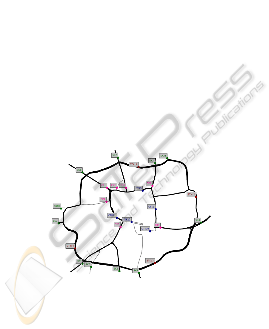
Figure 1 illustrates the cordons around the central part of the city. The stations
with the labels STK are on the ring road, and the stations with labels CK and CTK are
on roads through the city center. The network in the figure consists of all main roads.
Trips were defined as a sequence of measurements of the same license plate. We
used certain criterion to split sequences in separate trips when it was quite likely a
driver actually had multiple destinations. However, due to significant variations in
travel times, e.g. due to the unpredictability of traffic control phases encountered
during a trip, it is quite difficult to distinguish multiple trips when the time at an in-
termediate destination is short. Actually, this problem also plays an important role in
GPS data from which modelers want to identify different destinations and trip pur-
poses. In some cases, it will remain difficult to distinguish between a stop at a desti-
nation and a traffic related stop. Although we do not know the exact number of these
cases, they probably only constitute at most a few percent of all trips. For general
trends, this issue is therefore not very relevant. However, it may be important for
modeling route choice probability distributions. Probabilities for long routes may then
be overestimated, because some of them actually constitute multiple trips.
Fig. 1.
Network of main roads and monitoring stations (labels) for the central part of Enschede.
Because travel times between consecutive stations are quite variable, we used the
average travel time rather than the individual travel times. For each pair of consecu-
tive stations, we estimated the average travel time and standard deviation of all ob-
served trips containing that pair, irrespective of origin, destination or route. Due to
70
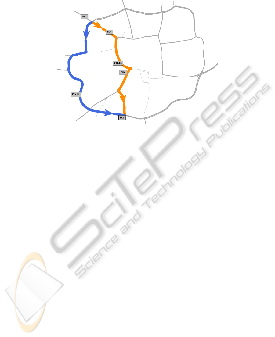
Fig. 2.
Observed routes for sequences between SK1 and SK6.
the large number of observations, average travel times are quite accurate. By adding
the average travel times between all consecutive stations in a sequence, the travel
time of the corresponding sequence was obtained.
For some individual trips, deviating travel times are the result of something atypi-
cal going on, for example, a driver who makes a stop at a petrol station or just an
error in the registration process. These so-called outliers were identified when the
travel time between two stations deviated more than 3 times the standard deviation
from the average travel time. As a result about 10% of trips were removed as outlier.
However, as suggested in the previous paragraph, some “bona fide” trips were proba-
bly also removed, while short activities in between two trips, like collecting or deliv-
ering someone or something, may not have been filtered out.
Figure 2 shows an example of the trips that were observed between station SK1
and SK6. The blue route is along the ring road, and the orange route through the city
center.
2.2 Route Set
Route assignment models use either implicit or explicit path generation. In explicit
path generation, the generation of the choice set and the assignment of choices (by
choice probabilities) are clearly distinct processes. Several authors (see for a review,
[18]) have argued that both should be done independently, because choice probabili-
ties may be affected by choice set size and composition.
However, even when paths are generated explicitly in advance, the alternatives
will always be biased in some way, because the modeler determines which “logical”
paths, i.e. those likely to be chosen, will be selected. For instance, large detours may
be perceived as illogical, but it is not certain whether they may not occur in some
71

cases. It is the purpose of route choice studies to reveal how likely both logical and
illogical routes are chosen in practice. This bias of using “a priori knowledge” may
even be enhanced when requirements are set to include used (observed) paths in the
route set, while equally valid unobserved paths may be left out. In such a bias against
“unseen” data, the occurrences of observed events are over estimated.
The aforementioned issues are in particular relevant for our survey. We do not ob-
serve paths. Instead, our so called observed routes only consist of sequences of moni-
toring stations. In between these locations, multiple paths are still possible. Fortunate-
ly, this problem can be dealt with, because the following is true for this survey. First,
most drivers take main roads. The use of residential streets is quite rare. Secondly,
between consecutive stations, there is often one unique path of main roads. If there
are multiple paths, these can be considered as overlapping, which means they are
actually considered as the same by the driver. Thirdly, different sequences are consid-
ered to be non-overlapping, because they contain different key intersections, which
make the corresponding routes quite distinct. Hence, each observed route (sequence
of links) can be represented by one unique underlying path.
Since link sequences represent unique paths, our route set only consists of link se-
quences. We do not need to know the paths, and therefore do not need a network of
roads. This will simplify the route set generation enormously, but also has the ad-
vantage that observed routes can mapped one-on-one to routes in the route set. An-
other advantage is that we almost do not need to make assumptions about the plausi-
bility of certain routes in advance. Thus, almost all possible routes are selected, in-
cluding unobserved routes. This means that we are careful not to introduce biases
against “unseen” or “illogical” routes.
We used a simple route set method in which new routes, i.e. sequences, were cre-
ated by appending stations to the last station of the previous sequence. Each sequence
only contained pairs of consecutive stations which also appeared in observed se-
quences. Also, (sub) circular routes were not allowed, and a time limit relative to the
shortest time route was used to stop the creation of very long alternatives. Yet, with
these restrictions still about 80 alternative routes per OD pair were found, which is
much more than in other route set generation methods.
2.3 Main Results
We found that most drivers use the shortest time route. However, 25% of the trips did
not use the shortest time route, but a detour route. This is quite a significant fraction,
but it is smaller than typically found in the literature, e.g. [13], [14], [15]. In those
studies, typically fewer than 50% of the drivers take the shortest time route. The dif-
ference may be related to the relatively “low resolution” of our data, which does not
allow us to distinguish different, but resembling, paths. On the other hand, the sam-
ples sizes of participants and corresponding OD pairs were relatively small (in order
of magnitude of 100) in the aforementioned studies. Moreover, in most studies the
samples only contained university staff members and / or commuters. Even if we
would consider the samples in these studies to be representative, they are far from
complete. It should be noted, however, that while our sample may be complete for the
city of Enschede, it only contains city trips and no highway trips. It is therefore not
72

unlikely that the sample differences may be responsible for differences in results.
For a subsample of OD pairs, which cut the city center, we found that even more
drivers, i.e. 88%, took the shortest time route when the ring road was faster than the
route through the center. However, we found that only 14% took the shortest time
route when the ring road was slower than the route through the center. Travelers thus
preferred the route along the ring road even if it was not the fastest route. For this
particular network constellation, road hierarchy appears to be crucial, and just as
important as travel time. We also conclude that it is only useful to compare route
choice fractions over shortest time routes when the context is the same.
Whereas route frequencies are quite sensitive to the characteristics of OD pairs,
overall detour times are much more robust. We found that the average detour time is
about 8% of the average travel time over the shortest time route. This results is quite
comparable with the literature, e.g. [14], [16]. This can be explained by the fact that
for OD pairs with only long alternative routes, a relatively small percentage of trips
over these alternatives will be offset by larger detour times for these alternatives.
3 Travel Time Estimates for Signalized Intersections
The municipality of Enschede has the objective to reduce the number of vehicle kil-
ometers by 5%. Consequently, the accessibility will be improved. For this purpose,
travelers may be given incentives to change their behavior. This can for example
already be done by confronting them with their “bad” travel behavior in comparison
with that of other travelers. Another way is to inform travelers about the traffic status,
and provide them with alternative modes or routes, which may yield more sustainable
trips.
In the latter case, travel times and volumes in the network should be estimated.
Travel times can be observed by floating car data, e.g. by GPS tracking. Roadside
systems can also be used to estimate travel times. For example, Bluetooth data may
provide quite reliable travel time estimates, e.g. [19]. We used data from inductive
loops near all important signalized intersections in Enschede to estimate travel times
or delays. These data were obtained from January 2010 till June 2011. Although
travel times can only be estimated in an indirect way by inductive loops, they provide
a complete dataset of all drivers who passed these intersections. They therefore also
provide volumes, which are typically not observed from GPS data alone. The ad-
vantage of volume measurements is that they enable an assessment on why travel
times deviate. In some cases, travel times increase, for example due to bad weather,
while volumes remain constant or even decrease. In other cases, for example at the
start of a normal rush hour, travel times increase due to increasing road volumes. If an
explicit distinction can be made between capacity and demand related travel time
deviations, this may yield more reliable short term travel time predictions.
3.1 Loop Data
A signalized intersection consists of 4 to 12 signal groups, indicated by the traffic
73
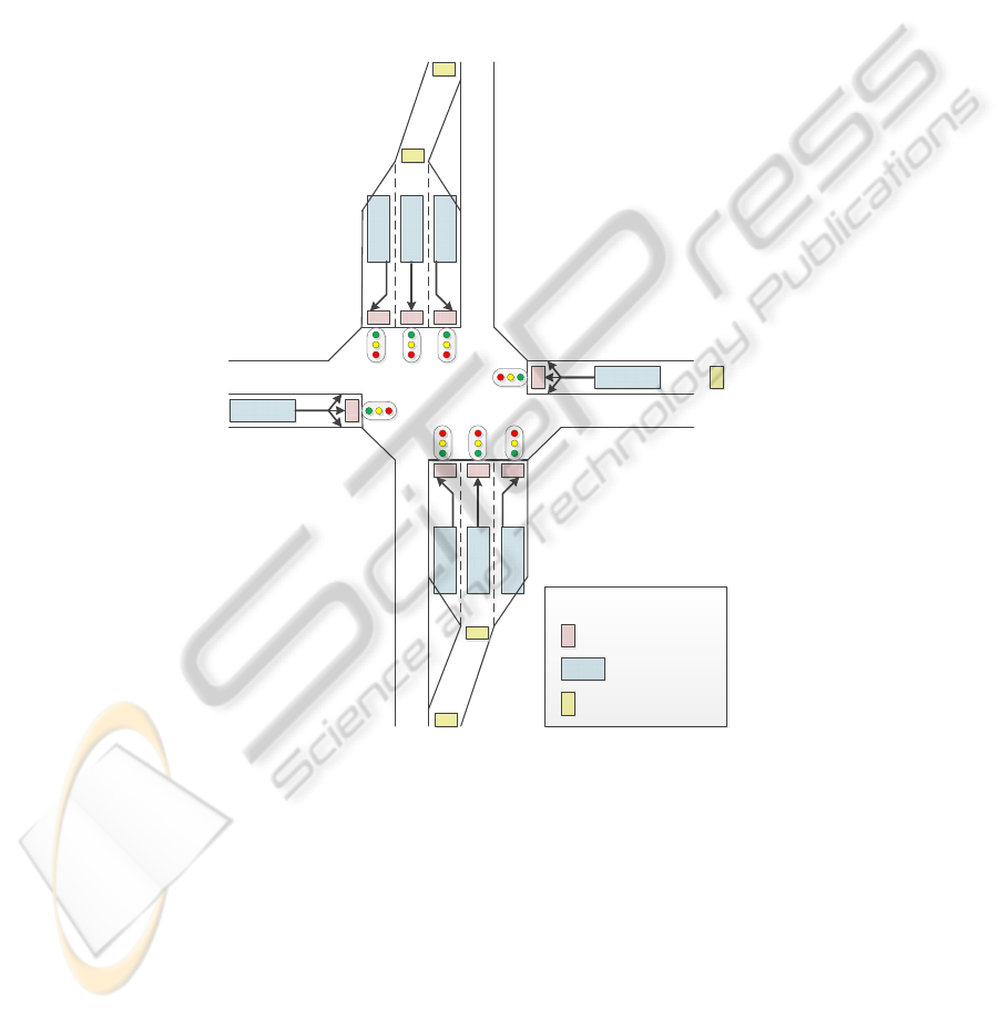
light symbols in figure 3. The figure shows that a signal group consists of 1 to 5 in-
ductive loops. The loops associated to a signal group all have particular functions.
The loop closest to the stop line (stop line loop) is mostly used to detect vehicles at
the stop line and to estimate the volume of vehicle passing through. The second loop
(long loop, if present) is generally situated 10 to 15 meters upwards from the stop line
and is used to detect the first hints of a queue. The other loops (distant loops) are used
to detect approaching vehicles. These loops can also be used to count the inflow of
vehicles at a particular arm of the intersection. Most inductive loops are connected to
one signal group, but distant loops can sometimes be associated with more than one
signal group.
Legend:
Stop line loop
Distant loop
Long loop
Fig. 3.
Example of an intersection and its inductive loops.
The data were aggregated in 5-minute intervals. For different types of loops the
data were further aggregated to the signal group level. Although we plan to use all the
data, especially for estimating delays of oversaturated flows, so far we only used
information from stop line loops. Flow volumes were estimated by adding vehicle
counts from stop line loops belonging to the same signal group, and signal group
occupancy rates were estimated as the weighted (by vehicle count) average over the
corresponding loops. Also, the total red time and number of times the signal group
74

switched from red to green were recorded. Finally, we also kept record of the occu-
pancy time during red as fraction of the total time (5 minutes).
Unreliable data were flagged. This was done as follows. If the volume was 0 or the
vehicle count of at least one loop exceeded a maximum limit, the observation was
flagged (flag = 0) as unreliable. The limit was set such that the time headway between
two vehicles during green time should not be smaller than 1.5 seconds. Smaller val-
ues are unrealistic and indicate rapid and artificial variation in the loop’s induction
current. A volume of 0 does not necessarily have to point to a malfunctioning of the
loops. In fact, in the middle of the night it is possible that no cars are passing during a
five minute period. However, it is no problem to flag these “bona fide” measure-
ments, because they are not relevant to the traffic manager, and cannot be used to
estimate the travel time anyway.
We mapped the signal groups to a network of roads. This enabled us to provide
route travel times by combining (free flow) travel times on road segments with the
estimated travel times or delays at the signalized intersections. For intersections with-
out measurements, we estimated the travel time by using a macroscopic traffic model.
3.2 Delay Estimation
Because delays cannot be measured directly from loop data, queuing theory is often
used to estimate delays, e.g. [20]. If we assume a homogenous arrival rate of vehicles
near saturation (green time is just sufficient to let all queuing vehicles through), the
average delay per vehicle is half the red time of one cycle. For a random arrival rate,
the delay increases somewhat, but the largest delays occur when cars arrive in clus-
ters, i.e. the intensity during arrival is the same as the discharge intensity. In other
words, all drivers will wait the same amount of time for a red traffic light. Near satu-
ration, this would yield an average delay of the red time of one cycle.
In figure 4, we show the case in which arrival intensities are the same as discharge
intensities for an arbitrary average 5 minute flow volume. The figure shows that all
cars have the same waiting time. Hence, the average delay is the delay of the first car
in the queue. This delay can be calculated by multiplying the occupancy rate during
‘red’ and the red time per cycle. Both quantities can be derived from the recorded
observations.
We deviated from standard assumptions in queuing theory, because urban traffic
flows are quite clustered. This may in particular be true when controls are vehicle
actuated, such is the case in Enschede. Both in quiet traffic conditions and conditions
near saturation, these estimations may therefore be quite accurate. For intermediate
conditions the delay is probably somewhat over estimated. These simple estimates
could therefore be improved by including a flow dependent factor between 0.5 and 1
for under saturated flows.
3.3 Accuracy of Delay Estimations
To test the accuracy of our delay estimates, we compared our estimates with other
data sources. For the city of Enschede, a database with average speed profiles based
75
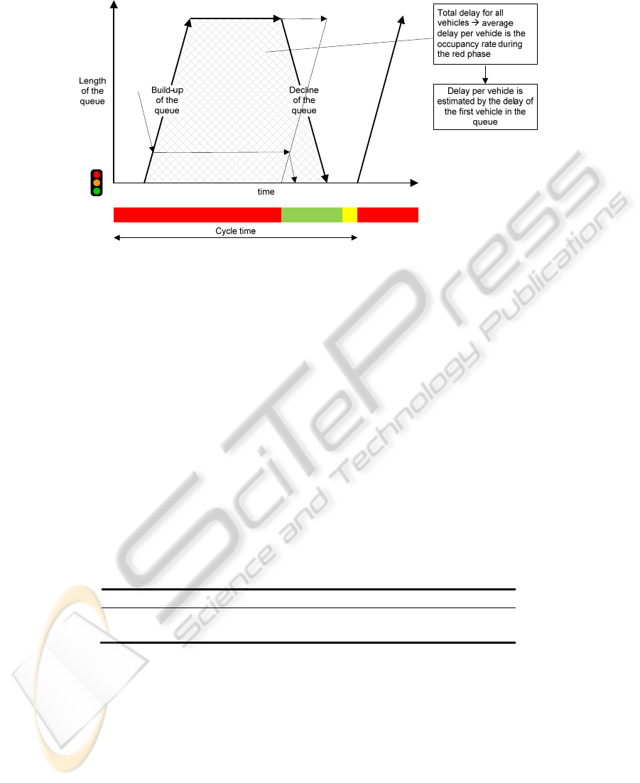
Fig. 4.
Illustration of queuing when cars in under saturated flows arrive in clusters.
on floating car data (called ViaStat) is available. From this database average travel
times on road sections can be extracted. We converted our delay estimates per signal
group into travel times by assuming free flow travel times on the corresponding road
segments. We chose the urban ring road for comparison. For both directions on the
urban ring road we estimated the travel time on an average Thursday morning peak
hour (between 8 and 9 AM).
In table 1, we show the comparison. The table suggests that our results are quite
valid. However, we should be careful interpreting these results. The comparison con-
sists of aggregates over many signal groups. Systematic errors in individual delays
could still be present. In particular, over estimation of delays in under saturated con-
ditions, could have been offset by an underestimation of delays in potential saturated
conditions. So far we did not consider saturated traffic conditions. In a saturated con-
dition the delays will increase dramatically when vehicles have to wait several cycle
times. For the estimations of these travel times, we might use data from previous 5
minute intervals to describe the growth of the queue, and apply correction factor
larger than 1 to capture the increasing delays.
Table 1. Travel times based on ViaStat and our estimates.
Based on ViaSTAT Our estimate
Ring road ‘right’
14 min 11 sec 13 min 35 sec
Ring road ‘left’
13 min 50 sec 14 min 11 sec
4 Urban Traffic Flow Predictions
One of the objectives is to generate accurate information on flow volumes and travel
times. Users need to be able to plan their journey based on this information. Thus not
only real-time information should be generated, but also predictions for the (near)
76

future. Different approaches exist for predicting volumes and travel times. Extrapola-
tion models (both spatial and temporal) are often used for short term predictions, e.g.
[21], [22]. Extrapolations can give accurate predictions, but only for prediction hori-
zons smaller than 15-20 minutes. For longer prediction horizons, volume measure-
ments can also be matched to historical patterns. For these predictions neural net-
works, e.g. [23], [24], or clustering methods, e.g. [25], [26], are applied.
4.1 Base-line Prediction
Autoregressive models (e.g. ARIMA models) are common in time-series forecasts.
Their forecasts are based on linear combinations of measurements from previous
time-intervals. Travel demand variations are often non-linear. Several authors, e.g.
[21], [22], [26], have therefore indicated that they prefer to use the average historical
profile of a whole day for predictions of a future day. In this case, non-linear features
may already be captured by the historical profile. Based on these results, our first
prediction for day d, link l and time interval t is equal to the historical mean of the
group to which day d belongs.
D
Dd
obs
ltd
dlt
base
dlt
n
q
qq
∑
∈
==
'
'
(1a)
D
Dd
obs
ltd
dlt
base
dlt
n
D
DD
∑
∈
==
'
'
(1b)
In equation (1a), we call
base
dlt
q the base-line prediction, and
obs
dlt
q
is the measured
volume on day d, link l and time interval t. Equation (1b) provides the base-line pre-
diction for delay D. Figure 5 illustrates base-line predictions for 5 minute intervals of
a particular traffic control during Mondays, Thursdays and Saturdays. The upper
panel shows significant day-to-day variation. The characteristic morning rush hour
peak is absent during Saturdays, while Thursdays show extra traffic in the evening
due to extra shopping hours. The lower panel shows the average delay for these
weekdays. The figure nicely illustrates that during busy periods, travel times also
increase.
4.2 Short Term Predictions
When large events take place traffic flows may be influenced by the visitors of these
events. At certain locations this will lead to a significant increase of traffic just before
the event has started and after the event has finished. These events should be taken
into account, implicitly by pattern recognition or explicitly by using historical data of
events and knowledge about the occurrence of a new event. However, base-line pre-
dictions sometimes also do not follow the measurements in a regular situation. Ap-
parently, traffic counts show systematic variations in time, which cannot be described
by the regular day-to-day variation alone. Such variations can have different causes,
77
Fig. 5. Volumes (upper panel) and delays (lower panel) for a specific intersection and per 5
minute interval averaged over all Mondays, Thursdays and Saturdays.
like for example seasonal effects, changing weather conditions or road works.
From a visual inspection of time-series, we suspect that a large amount of the vari-
ation between successive time-intervals is random. This variation is called noise. The
amount of noise is an important quantity. If the amount of noise increases, systematic
variations can be detected less easily. It also gives an under limit for the predictive
power, because noise cannot be predicted. Noise can have different causes. It can be
caused by the random arrival process of cars. This process results in different head-
ways between following cars, which is an important source of variation on highways.
In urban areas traffic flows are interrupted by traffic signals. However, if green times
of these signals are unknown, they may even contribute to the noise. In practice, all
variations which have short time-scales and which do not follow a recurrent pattern
can be considered as noise.
A measurement of quantity x on day d, at link l and in time interval t can thus be
described in the following terms:
dltdlt
pred
dlt
obs
dlt
xx
νε
++=
(2)
with
pred
dlt
x the prediction (e.g. the base-line prediction),
ε
dlt
the systematic variation
between measurement and prediction, i.e. the prediction error and
ν
dlt
the noise on
day d, at link l and in time interval t.
The objective is to develop a prediction scheme that minimizes the systematic var-
iation or prediction error. There are two extreme approaches to reach this objective.
First, the external processes that lead to systematic variations can be studied in detail,
so that the relation between the two can be modeled (e.g. the relation between weath-
er and travel demand). The advantage of this approach is that it provides insight in the
78

variation of travel demand. The disadvantage is that it is complicated and requires
many reliable data sources, which are often not available. Another approach is a
black-box approach. In this approach correlations in historical data are found by cer-
tain mathematical techniques (e.g. neural networks, pattern matching) and these cor-
relations are used in the prediction scheme.
We applied an intermediate approach. Our method is based on the following as-
sumption. The single most important temporal correlation in the systematic variation
is that between successive epochs (which can have different time-scales), i.e. there is
a positive correlation between the systematic variation
ε
dlt
and
ε
dlt+Δt
. For example,
due to seasonal effects, we assume that if there is more traffic than average on a par-
ticular day, than the probability is high that the next day will also show more traffic.
The improvement of the base-line prediction is quite simple in this case. The relative
systematic variation c (with
ε
= cq
pred
) results from the ratio between the observation
and base-line prediction. Suppose that this ratio is 1.10, i.e. c is estimated to be 10%.
Dependent on the strength of the correlation between the relative systematic variation
of successive time intervals, the updated prediction then lies between 1.00 (in case of
no correlation) and 1.10 (in case the correlation coefficient is 1) times the base-line
prediction.
Hence, the short term predictions up to 24h ahead can be described as:
q
dlt
dlt
tdlt
pred
tdlt
q
q
qq
β
⎟
⎟
⎠
⎞
⎜
⎜
⎝
⎛
=
Δ+Δ+
*
(3a)
D
dlt
dlt
tdlt
pred
tdlt
D
D
DD
β
⎟
⎟
⎠
⎞
⎜
⎜
⎝
⎛
=
Δ+Δ+
*
(3b)
In which the base-line prediction at t + Δt is updated by the ratio between real-time
observations and base-line predictions at t. We used hourly volumes to estimate this
ratio. In doing so, we reduced the influence of noise, while still capturing most of the
changes in the systematic variation. As mentioned, the update factor β depends on the
strength of the correlation between the relative systematic variation at t and t + Δt. In
Figure 6, we show the relative systematic variation of successive days for volumes
(upper panel) and delays (lower panel) for a particular traffic control. We did this for
each hour of the day between 6.00 and 22.00h. The figure shows positive correlations
(with correlation coefficient 0.79 for volumes and 0.68 for delays). The correlation is
less strong for the delay, because of the larger amount of noise in the delay estima-
tions. These correlations yield βs of around 0.7.
Besides seasonal influences, which can be used to make predictions on a longer
timeframe (i.e. one to two days ahead), real-time data may be used to improve predic-
tions for shorter time horizon. We estimated the correlation between systematic varia-
tion in successive hours, and found these to be comparable to that of successive days.
These are still preliminary results. Due to the high noise level, in especially delay
estimates, systematic variations are not easily resolved. As a result, at the moment
short term predictions are only slightly better than base-line predictions. However,
short term predictions can be improved when the noise in the observations are filtered
[27]. Without a noise filter, the quality of the prediction quickly reaches an upper
limit set by the amount of noise in the observations.
79
Fig. 6. Correlation between relative systematic variations of successive days for volumes (up-
per panel) and delays (lower panel).
5 Discussion
Traffic management has developed significantly in the last few decades. However,
especially for urban areas, future developments are required.
The first development concerns monitoring. Network wide measures can only be
effective if the traffic situation is monitored throughout the whole network. This
poses a challenge. Roadside sensors do not always cover the whole network. For
example, in sections 3 and 4 we used data from detection loops to monitor the traffic
situation in the Dutch city of Enschede. Because some (important) intersections are
not equipped with sensors, our estimates and forecasts are incomplete. Ideally, road-
side measurements could be supplemented by floating car data, e.g. by GPS, from
individual travellers. GPS data alone are probably not sufficient either, because traffic
is quite dispersed in urban networks, which implies GPS data from a high fraction of
motorists are needed. A fusion between the different data types might be the solution,
and could be one of the challenges in a new project.
Floating car data may also be used to improve travel time estimates throughout the
network. We used a quite simple algorithm to estimate delays at signalized intersec-
tions using occupation rates and red times. However, in particular for saturated condi-
tion, delays are probably underestimated by this simple method. We therefore need to
improve the travel time algorithm. In addition, car floating data can be useful for
validation purposes.
Monitoring in itself is not sufficient. Predictions about the traffic situation enable
controllers to anticipate on the (near) future, such that timely measures to control the
80

amount of traffic in one part of the network may prevent bottlenecks in other parts. In
section 4, we used a simple prediction algorithm to forecast volumes and travel times
in the near future. The predictions can however be improved. First, noise filters could
reduce the noise in the observations and as a result yield better predictions. Secondly,
so far we only considered single time series. However, volumes and delays may be
spatially correlated. We might improve the predictions by including spatial correla-
tions between sensors, but this will only be effective when most adjacent intersection
are equipped with sensors. Unfortunately, this is not always the case. Finally, we
focus on slow changing systematic variations in traffic. However, for managers, sud-
den changes due to events or incidents are often more relevant. The related traffic
situations may in those cases be better predicted by pattern matching algorithms. It
may be possible to develop a hybrid method, which combines pattern matching and
forecasts of slow changing variations.
The second development concerns personalized traffic control. Predictions are not
only useful for traffic control managers, but also for road users. If they are informed
about future traffic flows and control strategies, they may make choices that enhance
those strategies. This will only be possible if personal needs and expectations of road
users are taken into account by traffic control strategies.
For this purpose, we need to explore travel behavior. We used a license plate sur-
vey to study route choice in the municipality of Enschede. We found that most drivers
use the shortest time route, but that 25% of the trips did not use the shortest time
route. Moreover, we found that most travellers took the ring road instead of the route
through the city centre, even when the ring road was slower. This result suggest that
travellers do not need to take the fastest route, but that they may prefer larger roads
(higher up in the hierarchy). Many traffic managers would like to see drivers to take
the ring road instead of small roads through the city center. These results suggest that
strategies to increase the use of ring roads are probably acceptable to users and may
also be quite successful.
References
1. Hasberg, P., Serwill, D.: Stadtinfoköln – a global mobility information system for the
Cologne area, 7
th
World Congress on Intelligent Transport Systems, Turin, Italy (2000)
2. Kellerman, A., Schmid, A.: Mobinet: Intermodal traffic management in Munich –control
centre development, 7
th
World Congress on Intelligent Transport Systems, Turin, Italy
(2000)
3. Leitsch, B.: A Public-privat partnership for mobility – Traffic management Center Berlin,
9
th
World Congress on Intelligent Transport Systems, Chicago (2002)
4. Nagatani, T.: Vehicular traffic through a sequence of green-wave lights, Physica A: Statis-
tical Mechanics and its Applications, Vol. 380, (2007) 503-511
5. Vrancken, J., Van Schuppen, J.H., Dos Santos Soares, M., Ottenhof, F.: A
HierarchicalNetwork Model for Road Traffic Control, Proceedings of the 2009 IEEE Inter-
national Conference on Networking, Sensing and Control, Okyama, Japan, (2009) 340-344
6. Hodge, V.J., Krishnan, R., Jackson T., Austin, J., Polak, J.: Short Term Traffic Prediction
Using a Binary Neural Network, 43rd Annual UTSG Conference, Open University, Milton
Keynes, UK (2011)
81

7. Wismans, L.J.J, Van Berkum, E.C., Bliemer, M.C.J.: Comparison of Evolutionary Multi
Objective Algorithms for the Dynamic Network Design Problem. ICNSC – IEEE confer-
ence, Delft (2011)
8. Mitsakis, E., Salanova, J.M., Giannopoulos, G.: Combined dynamic traffic assignment and
urban traffic control models, Procedia - Social and Behavioral Sciences, Vol. 20, (2011)
427 – 436
9. Wardrop, J. G.: Some theoretical aspects of road traffic research, Proceedings, Institute of
Civil Engineers, PART II- 1, (1952) 325-378.
10. Bar-Gera, H., Mirchandani, P., Fan, W.: Evaluating the assumption of independent turning
probabilities, Transportation Research part B, Vol. 40, (2006) 903 - 916
11. Chen, T.Y., Chang, H.L., Tzeng, G.H.: Using a weight-assesing model to identify route
choice criteria and information effects, Transportation Research Part A, Vol. 35, (2001)
197 – 224
12. Mahmassani, H.S., Jou, R-C.: Transferring insights into commuter behavior dynamics from
laboratory experiments to field trials. Transportation Research Vol. 34A(4), (2000) 243-
260
13. Prato, C. G., Bekhor, S.: Applying Branch-and-Bound Technique to route choice set gener-
ation. Transportation Research Record, Vol. 1985, (2006) 19-82
14. Jan, O., Horowitz, A. J., Peng, Z. R.: Using global positioning system data to understand
variations in path choice. Transportation Research Record, Vol. 1725, (2000) 37 – 44.
15. Zhu, S., Levinson, D.: Do people use the shortest path? An empirical test of Wardrop’s first
principle, 4th International Symposium on Transportation Network Reliability, July Min-
neapolis, USA (2010)
16. Papinski, D., Scott, D. M.: A GIS Toolkit for route choice analysis, Journal of Transport
Geography, Vol. 19, (2009) 434 – 442
17. Hamerslag R.: Investigation into factors affecting the route choice in “Rijnstreek-West”
with the aid of a disaggregate logit model. Transportation, Vol. 10, (1981) 373 – 391.
18. Bovy, P. H. L.: On modeling route choice sets in transportation networks: a synthesis,
Transport Reviews, Vol. 29 (1), (2009) 43 – 68
19. Tarnoff, P. J., Wasson, J. S, Young, S. E., Ganig, N., Bullock, D. M., Sturdevant, J. R.: The
Continuing Evolution of Travel Time Data Information Collection and Processing, Trans-
portation Research Board Annual Meeting, Paper ID: 09-2030 (2009)
20. Mak, W. K., Viti, F., Hoogendoorn, S. P., Hegyi, A.: Online travel time estimation in urban
areas using the occupancy of long loop detectors, 12th IFAC symposium on transportation
systems, Redondo Beach (2009)
21. Wild, D.: Short-term forecasting based on a transformation and classification of traffic
volume time series, International Journal of Forecasting, Vol. 13, (1997) 63 – 72
22. Van Grol, R., Inaudi, D., Kroes, E.: On-line traffic condition forecasting using on-line
measurements and a historical database, 7
th
World Congress on Intelligent Transport Sys-
tems, Turin, Italy (2000)
23. Dia, H.: An object-oriented neural network approach to short-term traffic forecasting,”
European Journal of Operational Research, Vol. 131, (2001) 253 – 261
24. Yin, H., Wong, S. C., Xu, J., Wong, C. K.: Urban traffic flow prediction using a fuzzy-
neural approach, Transportation Research Part C, Vol. 10, (2002) 85 – 98
25. Chung E.: Classification of traffic pattern, 10
th
World Congress on Intelligent Transport
Systems, Madrid (2003)
26. Weijermars, W. A. M,: Analysis of urban traffic patterns using clustering, Ph.D. Thesis,
University of Twente, Enschede, The Netherlands (2007)
27. Thomas, T., Weijermars, W. A. M, Van Berkum E.C.: Predictions of Urban Volumes in
Single Time Series, IEEE Transactions on Intelligent Transportation Systems, Vol. 11 (1),
(2010) 71 – 80
82
