CONCATENATION METHOD FOR HIGH-TEMPORAL

RESOLUTION SSVEP-BCI

Yohei Tomita

, Antoine Gaume

, Hovagim Bakardjian

, Monique Maurice

2,3

, Andrzej Cichocki

Yoko Yamaguchi

, G´erard Dreyfus

and Franc¸ois-Benoˆıt Vialatte

1,2

SIGMA Laboratory,

Ecole Sup´erieure de Physique et de Chimie Industrielles de la Ville de Paris

10 Rue Vauquelin 75231, Paris Cedex 05, France

Riken BSI, Laboratory ABSP, 2-1 Hirosawa, Wako-shi, Saitama-Ken, 351-0128, Japan

Riken BSI, Laboratory DEI, 2-1 Hirosawa, Wako-shi, Saitama-Ken, 351-0128, Japan

Keywords:

Concatenation method, Heisenberg-Gabor uncertainty principle, High-temporal resolution BCI, SSVEP,

EEG.

Abstract:

Electroencephalographic (EEG) signals are generally non-stationary, however, nearly stationary brain re-

sponses, such as steady-state visually evoked potentials (SSVEP), can be recorded in response to repeti-

tive stimuli. Although Fourier transform has precise resolution with long time windows (5 or 10 s for in-

stance) to extract SSVEP response (1-100 Hz ranges), its resolution with shorter windows decreases due to the

Heisenberg-Gabor uncertainty principle. Therefore, it is not easy to extract evoked responses such as SSVEP

within short EEG epochs. This limits the information transfer rate of SSVEP-based brain-computer interfaces.

In order to circumvent this limitation, we concatenate EEG signals recorded simultaneously from different

channels, and we Fourier analyze the resulting sequence. From this constructed signal, high frequency res-

olution can be obtained with time epochs as small as only 1 s, which improves SSVEPs classiﬁcation. This

method may be effective for high-speed brain computer interfaces (BCI).

1 INTRODUCTION

Brain computer interfaces (BCI) are alternative meth-

ods to the normal outputs of the brain via the nerve-

muscle system (Birbaumer, 2006). The purpose of

BCI is to detect physiological signals from the brain

and translate them into a control signal for an external

device. It has been developed with surface electroen-

cephalograms (EEG), electrocorticograms (ECoG),

and implanted electrodes. Among them, surface EEG

has many advantages: it is non-invasive, technically

less demanding, and evoked responses are fast (within

the millisecond range). Especially, short response

times of EEG could enable users to control an ex-

ternal device almost in real-time (Sanei and Cham-

bers, 2007; Bashashati et al., 2007; Lotte et al.,

2007). However, nowadays the available BCI systems

are generally constrained to execute commands using

epochs of more than 3 s. For instance, in BCI word

processing systems, it takes more than 3 s to type each

letter. Therefore, being able to detect BCI commands

with shorter time epochs (about 1 s) is a crucial prob-

lem.

EEG signals are known to be non-stationary

(see

for instance (Kawabata, 1973)). However, in steady-

state visually evoked potentials (SSVEP), EEG fea-

tures at the stimulation frequency and its harmonics

are nearly stationary (Vialatte et al., 2010). When

subjects focus attention on ﬂickering lights with con-

stant frequencies, steady-state brain activity appears,

predominantly in the occipital cortex, and propagates

to other brain areas. These responses are better ob-

served in the frequency, or time-frequency domains.

Therefore, to detect these features, frequency or time-

frequency analysis methods are applied, such as clas-

sical Fourier transform or wavelet transform (Quiroga

et al., 2001; Vialatte et al., 2008; Bin et al., 2009).

Moreover there are other methods such as empiri-

cal mode decomposition for instantaneous frequency

(Huang et al., 1998).

To detect these SSVEPs with high temporal res-

olution, one generally uses short EEG epochs to

Their statistical properties evolve with time

444

Tomita Y., Gaume A., Bakardjian H., Maurice M., Cichocki A., Yamaguchi Y., Dreyfus G. and Maurice F..

CONCATENATION METHOD FOR HIGH-TEMPORAL RESOLUTION SSVEP-BCI .

DOI: 10.5220/0003724404440452

In Proceedings of the International Conference on Neural Computation Theory and Applications (Special Session on Challenges in Neuroengineering-

2011), pages 444-452

ISBN: 978-989-8425-84-3

 2011 SCITEPRESS (Science and Technology Publications, Lda.)

compute Fourier transforms. However, due to the

Heisenberg-Gabor uncertainty principle, high fre-

quency resolution cannot be obtained by Fourier

transforming short signals: the shorter the window

length, the lower the frequency resolution. Further-

more, when using short epochs, EEG becomes nearly

stationary. Therefore for short epochs the Fourier rep-

resentation of SSVEP and non-SSVEP activity are of

comparable amplitudes, hence SSVEP peak is difﬁ-

cult to be detected. As a result, SSVEP cannot be de-

tected reliably with short windows (a minimum of 3 s

is usually required). To circumvent this limitation, we

propose a concatenation method: EEG epochs mea-

sured simultaneously from different channels are con-

catenated, in order to generate an artiﬁcially longer

epoch that can be analyzed with a better frequency

resolution. The details of this method are described

in the following sections. We then demonstrate this

method on a real SSVEP classiﬁcation task.

The organization of the paper is as follows. Sec-

tion 2 details the procedure of the concatenation

method. In section 3, an EEG electrode placement

and the experimental procedure are presented. Re-

sults, discussions and conclusions are in sections 4, 5,

and 6, respectively.

2 CONCATENATION METHOD

In this section, the concatenation method is detailed.

Firstly, the non-stationarity of EEG is shown with dif-

ferent sizes of time epoch. Secondly, we propose the

concatenation method to circumvent this problem.

2.1 Non-stationarity of EEG

EEGs are considered non-stationary. When using fre-

quency analysis methods such as the Fourier trans-

form and the wavelet transform, rhythmic compo-

nents of the EEG (such as the theta or the alpha wave)

are extracted for decomposing a signal into a set of

frequency components. However, the Fourier trans-

form relies on the assumption that the analyzed sig-

nal is strictly stationary, otherwise, the resulting spec-

trum will make little physical sense. Therefore, when

using long time epochs, these non-stationary compo-

nents have limited impact on the Fourier spectrum.

On the other hand, when using short time windows,

EEG frequency components become nearly station-

ary, with higher resulting Fourier amplitudes.

SSVEPs are nearly stationary evoked responses,

much more stable than classical EEG signals. They

have very narrow-band responses, with precise spec-

tral properties (an SSVEP response at 10 Hz exhibit

0 2 4 6 8 10

−5

Oz signal

Amp.

Time (s)

5 10 15 20 25 30 35 40

500

Fourier power with 10 s window

Frequency (Hz)

5 10 15 20 25 30 35 40

500

Fourier power with 5 s window

Frequency (Hz)

5 10 15 20 25 30 35 40

200

400

Fourier power with 2 s window

Frequency (Hz)

5 10 15 20 25 30 35 40

100

200

Fourier power with 1 s window

Frequency (Hz)

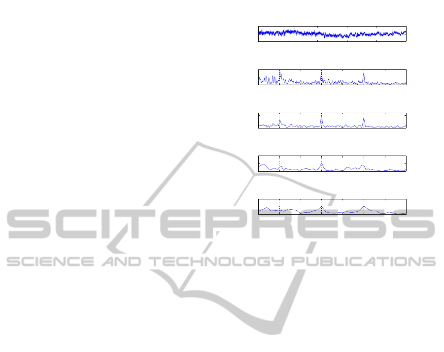
Figure 1: 10 Hz SSVEP responses: Top, Oz signal; Bot-

tom four, Fourier power with different time windows of [0,

time] (time∈[10, 5, 2, 1]). With the shorter windows, it

shows lower time resolution and the peak is lower at the

fundamental and harmonic frequencies.

a clear peak at 10 Hz, with a width below 1 Hz).

These responses can be observed in a frequency do-

main shown in Fig. 1.

Frequencies of EEG signal were calculated by

Fourier transform with different sizes of Hanning

window function. The spectrum obtained with a 10

s time window exhibits sharp peak nears 10, 20, and

30 Hz. Conversely, the spectrum obtained with a 1

s time window exhibits lower peaks at these frequen-

cies, and it has a lower frequency resolution. Notably,

Fourier powers at frequencies surrounding stimulus

frequency and its harmonics are higher when the time

epoch is shorter. This is because, for long EEG

epochs, the non-stationary components of EEG sig-

nals except the stimulus frequency have less impact

on the Fourier spectrum. Thus, sharper and clearer

SSVEP peaks can be obtained. On the other hand, for

short EEG epochs, it has lower spectral amplitudes,

which blurs out the SSVEP peak, which is further-

more distorted by the low frequency resolution.

2.2 Concepts of Concatenating

The concatenation method we propose is a way to im-

prove artiﬁcially the frequency resolution while using

very short EEG epochs. The details of this method are

as follows.

Let x

be the column vector of an signal observed

in the ith channel. The concatenated signal y is con-

CONCATENATION METHOD FOR HIGH-TEMPORAL RESOLUTION SSVEP-BCI

445

5 10 15 20 25 30 35 40

100

200

Fourier power of Oz signal

Frequency (Hz)

5 10 15 20 25 30 35 40

100

200

Mean Fourier power of O1, Oz, and O2 signal

Frequency (Hz)

5 10 15 20 25 30 35 40

200

400

Fourier power of Concatenated signal

Frequency (Hz)

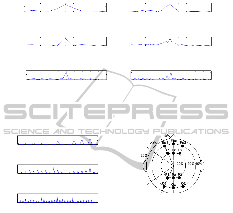
Figure 2: Frequency features of concatenated signal: Top,

Fourier power |X

jω

; Middle, mean Fourier power of

cha

jω

(cha = [O1, Oz,O2]); Bottom, Fourier power

|Y(e

jω

from a concatenated signal of O1, Oz, and O2.

structed by concatenating signals in the time domain:

y = [x

,...,x

]

, (1)

where M is the number of concatenated signals and T

represents transposition. If each signal is of length N,

then y is of length MN. Furthermore, let X

jω

) (resp

Y(e

jω

)) be the Fourier transform of x

(resp. y). Fre-

quency resolution of Y(e

jω

) is M times higher than

that of X

jω

). It can be explained by the larger size

of y. Using ω = 2π f (f is frequency), short time

Fourier transforms of these signals are expressed as

jω

) = X

2π j f

) =

N−1

∑

t=0

[t]e

−2π j ft

(2)

and

Y(e

jω

) = Y(e

2π j f

) =

MN−1

∑

t=0

y[t]e

−2π j ft

, (3)

where

f =

[Hz] (k∈N), (4)

and t and L represent time index and the time length

of 1 s, respectively. k represents the number of cy-

cles of a sinusoidal signal within the time window of

the Fourier transform. e

jω

should be 0 at the begin-

ning and the end of the epoch. Frequency resolutions

therefore are divided by the number of concatenations

As an example, EEG electrodes are attached at Oz,

O1, O2, Pz, P1, and P2 according to the international

10/20 system. SSVEP of all signals are measured

while 10 Hz visual stimulus is displayed. x

, x

and x

correspond raw signals at Oz, O1, and O2,

for instance. Concatenated signal y can be deﬁned

like [x

]. Here, we consider signals

, and y ([x

). Time length of each

EEG signal x

is 1 s (1 s epoch). In the Fig. 2, Fourier

power |X

jω

has weak peaks around 10 and 20

Hz. The mean of |X

cha

jω

(cha = [O1,Oz,O2])

has similar peak of |X

jω

. Contrary to that,

Fourier power of concatenated signal |Y(e

jω

has

stronger peak near 10 and 20 Hz.

Furthermore, we investigate effects of the num-

ber of signals: x

, y

([x

]

), y

([x

]

). With these

signals, Fig. 3 shows Fourier power |X

jω

, |Y

jω

in two different conditions: x

is 1 s or 2 s length. The Hanning window is of

length MN. From the ﬁgure, regardless of 1 s epoch

and 2 s epoch, the peak at 10 Hz appears more and

more clearly as the number of concatenated signals

increases. Thus, the concatenation method can ex-

tract sharper peak of SSVEP despite of short time

epoch. Furthermore, different window functions can

be used: no window function, Hanning window of

same length as the concatenated signal, or Hanning

window of same length as each signal, respectively.

In Fig. 3, Hanning window of same length as the con-

catenated signal is applied and it is also used in the

next sub-section.

Finally, concatenation of a EEG signals repetively

were investigated. It uses only one EEG signal.

This concatenated signal is expressed as y

same

,...,x

]

. Fourier powers of this signal with

different time epochs are shown in Fig. 4. These are

small peaks at 1 Hz interval in Fig. 4-(a), 0.5 Hz inter-

vals in Fig. 4-(b), and 0.2 Hz intervals in Fig. 4-(c). It

may be a problem for detection of SSVEP peaks. It is

obviously explained by the property of Fourier trans-

form (see APPENDIX). Therefore, concatenation of

EEG signals from different channels conduces better

observation of SSVEP peaks.

3 EXPERIMENTAL

DEMONSTRATION

Eight subjects took part in the experiment, and signed

written informed consent forms. EEG signals were

taken from a database recorded during SSVEP stimu-

lation in Riken BSI/Japan. Photic stimulation is given

using AVOTEC goggles and the ﬂickering frequency

is controlled by a shutter which allows a maximal re-

freshing rate of 293 Hz. A very broad range of fre-

quencies is recorded (21 different frequencies from

1 Hz to 100 Hz): 1.00, 1.25, 1.88, 2.50, 3.33, 4.17,

NCTA 2011 - International Conference on Neural Computation Theory and Applications

446

5 6 7 8 9 10 11 12 13 14 15

200

Frequency (Hz)

Power

5 6 7 8 9 10 11 12 13 14 15

500

Frequency (Hz)

Power

(a1)1sepoch,onesignal (b1)2sepoch,onesignal

5 6 7 8 9 10 11 12 13 14 15

500

Frequency (Hz)

Power

5 6 7 8 9 10 11 12 13 14 15

500

Frequency (Hz)

Power

(a2)1sepoch,twosignals (b2)2sepoch,twosignals

5 6 7 8 9 10 11 12 13 14 15

1000

Frequency (Hz)

Power

5 6 7 8 9 10 11 12 13 14 15

1000

2000

Frequency (Hz)

Power

(a3)1sepoch,sixsignals (b3)2sepoch,sixsignals

Figure 3: Frequency features of concatenated signal: Left three ﬁgures, length of each EEG signal is 1 s (1 s epoch); Right

three ﬁgures, length of each EEG signal is 2 s (2 s epoch); Top two ﬁgures, Fourier power |X

jω

; Middle two ﬁgures,

Fourier power |Y

jω

is of Oz and O1); Bottom three ﬁgures, Fourier power |Y

jω

is of Oz, O1, O2, Pz, P1,

and P2).

5 6 7 8 9 10 11 12 13 14 15

500

1000

Frequency (Hz)

Power

(a) y

same

,1sepoch,eightsignal

5 6 7 8 9 10 11 12 13 14 15

1000

Frequency (Hz)

Power

(b) y

same

,2sepoch,eightsignals

5 6 7 8 9 10 11 12 13 14 15

1000

2000

Frequency (Hz)

Power

same

,5sepoch,eightsignals

Figure 4: Frequency features of y

same

with eight same sig-

nals: Top, 1 s epoch; Middle, 2 s epoch; Bottom, 5 s epoch.

5.00, 6.67, 8.33, 10.00, 13.33, 16.67, 20.00, 26.67,

33.33, 40.00, 53.33, 66.67, 80.00, 90.00, and 100.00

Hz. Firstly a subject sees a uniform grey screen for

20 s, then a ﬂickering stimulus for 10 s, and then iter-

atively restarts this sequences of rest/stimulus condi-

tion. Stimuli were presented in a randomized order, in

seven runs of nine frequencies, for a total of 63 trials

(3 trials per 21 frequency).

EEG was recorded using a Biosemi system in a

shielded room, with 128 active channels, all signals

were ampliﬁed and digitized at 1024 Hz, after ana-

log ﬁltering of frequencies above 100 Hz and notch

ﬁltering at 50 Hz.

In this paper, parts of EEG channels are used as

Figure 5: A placement of electrodes which are used for

analysis in this paper.

shown in Fig. 5 (12 EEG channels: Fp1, Fpz, Fp2,

F1, Fz, F2, P1, Pz, P2, O1, Oz, and O2) and visual

stimuli of 10 and 13.33 Hz are used to investigate ef-

fectiveness of the concatenation method.

4 RESULTS

In this section, SSVEPs evoked by 10 and 13.33 Hz

stimuli are investigated. First of all, EEG features to

classify the SSVEPs are detailed. Then, SSVEPs of

10 and 13.33 Hz are classiﬁed with several features

selected by a supervised feature ranking method, the

Gram-Schmidt orthogonalization. Finally, we com-

pare the frequency domain of a concatenated signal

with that of the signals which are used for concatena-

tion.

CONCATENATION METHOD FOR HIGH-TEMPORAL RESOLUTION SSVEP-BCI

447

4.1 EEG Feature Extraction

SSVEP responses have peaks at the stimulus fre-

quency and even harmonics (Fig. 1). Using 10 and

13.33 Hz as stimulus frequencies, SSVEPs are de-

scribed by six different features for the purpose of

classiﬁcation: ξ

, the spectral power at the stimu-

lation frequency; ξ

, the frequency power enhanced

by SSVEP SNR (Vialatte et al., 2010) applied to the

frequency domain; ξ

, the magnitude square coher-

ence function between two signals; ξ

, global ﬁeld

synchronization; ξ

and ξ

, the frequency power and

SSVEP SNR of the concatenated signals.

The ﬁrst feature is deﬁned as

( f ) = |X( f)|

+ |X( f×2)|

, (5)

i.e. sum of the spectral powers of the fundamental

and its ﬁrst harmonic. This feature is extracted at

each channel of both 10 and 13.33Hz. Although ξ

has similar feature with ξ

, SSVEP peaks can be en-

hanced by SSVEP SNR as

′

( f ) =

nX( f)

∑

n/2

k=s

X( f + k△ f) +

∑

n/2

k=s

X( f − k△ f)

, (6)

and then the second feature can be deﬁned as

( f ) = |X

′

( f )|

+ |X

′

( f ×2)|

. (7)

The coherence function, a synchrony measure, is

distinguished into the magnitude square coherence

function and the phase coherence function (see for in-

stance (Nunez et al., 1997; Dauwels et al., 2010)).

Magnitude square coherence function is the third fea-

ture we used. It is deﬁned as

i, j

( f ) =

( f )X

∗

( f )|

( f )||X

( f )|

, (8)

where X

∗

is the complex conjugate of X, i and j cor-

respond to the label of channel. It is a function of two

signals, therefore, the number of pairs of all channels

corresponds to the number of combinations.

Similarly, global ﬁeld synchronization (GFS),

another synchrony measure, is the fourth fea-

ture. GFS quantiﬁes the synchrony of multi-

ple signals. First of all, with Fourier trans-

formed signals, one constructs the vectors X

( f ) =

(Re(X

( f )),Re(X

( f )),...,Re(X

( f )))

and X

( f ) =

(Im(X

( f )),Im(X

( f )),...,Im(X

( f )))

, and com-

putes the covariance matrix C∈R

2×2

for those two

vectors. GFS (ξ

( f )) is deﬁned in terms of the nor-

malized eigenvalues λ

and λ

of C:

( f ) = λ

− λ

. (9)

Finally, with concatenated signals, the Fourier

power and SSVEP SNR are deﬁned as

( f ) = |Y( f )|

+ |Y( f×2)|

, (10)

( f ) = |Y

′

( f )|

+ |Y

′

( f ×2)|

. (11)

Here, we used six groups of channels for concatena-

tion: (Fp1-Fpz-Fp2), (F1-Fz-F2), (P1-Pz-P2), (O1-

Oz-O2), (Fp1-Fpz-Fp2-F1-Fz-F2), and (P1-Pz-P2-

O1-Oz-O2).

There are six different features with different pa-

rameters. There are parameters of two stimulus fre-

quencies and the channel locations for all features;

and the window functions, and channel groups which

are only for concatenated feature. We prepared two

different conditions:

1. Condition 1 includes the Fourier, SSVEP SNR,

coherence and GFS feature. In this condition,

the total number of feature is 24(ξ

) + 24(ξ

) +

132(ξ

) + 2(ξ

) = 182.

2. Condition 2 includes the Fourier and SSVEP SNR

of each EEG signal, that of the concatenated sig-

nals, coherence and GFS feature. In this con-

dition, the total number of features is 24(ξ

) +

24(ξ

) + 132(ξ

) + 2(ξ

) + 24(ξ

) =

230.

4.2 SSVEP Classiﬁcation

For classifying the SSVEPs, the number of features

must be as small as possible (see for instance (Drey-

fus, 2005)). Input ranking thorough Gram-Schmidt

orthogonalization is applied to select all relevant fac-

tors as inputs to the classiﬁer, but only the relevant

ones. The relevance is measured by the angle between

the vector of a feature (ξ

) and the vector of stimuli la-

bel (l) as

cos

|(ξ

)

|(ξ

)

ξ||l

. (12)

Firstly, a feature which is most correlated to the fea-

ture (l) is chosen by the largest cos

. l and all other

candidate inputs are projected onto the null space of

the selected input (subspace). The above procedure

is iterated until all features have been ranked. With

ranked features, SSVEPs are classiﬁed by linear dis-

criminant analysis (LDA). Performances are deﬁned

as the classiﬁcation accuracy (ACC) calculated with

leave one out cross validation (LOOCV). These pro-

cedures are applied for two cases (two frequencies):

using all features except concatenation features (Con-

dition 1) and using all features (Condition 2). Addi-

tionally, we use four different time epochs (1.0, 2.0,

5.0, 10.0 s).

Table 1 shows ranked top 10 features thorough

Gram-Schmidt orthogonalization. These results are

performed with 1 s epoch. Mostly, ξ

, ξ

with

different parameters are chosen when concatenation

NCTA 2011 - International Conference on Neural Computation Theory and Applications

448

Table 1: Feature ranking with 1 s epochs: FT represents ξ

, SNR represents ξ

, MC represents ξ

, ConcateFT represents

, and ConcateSNR represents ξ

. The ranking is calculated ﬁrstly without the concatenation features (Condition 1), then

including them (Condition 2). Concatenation features were chosen in high ranks.

Rank Condition 1 Condition 2

(without councatenation) (with councatenation)

1 FT (P22, 13.33 Hz) ConcateFT (group6, 10 Hz, window2)

2 FT (F2, 10 Hz) ConcateFT (group2, 13.33 Hz, window1)

3 SNR (Oz, 13.33 Hz) ConcateSNR (group6, 10 Hz, window1)

4 SNR (O2, 10 Hz) SNR (O2, 10 Hz)

5 MC (F1-P2, 10 Hz) ConcateSNR (group3, 13.33 Hz, window3)

6 MC (F1-P2, 13.33 Hz) ConcateSNR (group2-1, 13.33 Hz, window3)

7 MC (Fpz-P1, 10 Hz) MC (F1-P2, 10 Hz)

8 MC (Fpz-F2, 13.33 Hz) MC (Fpz-P1, 10 Hz)

9 MC (Fp2-Oz, 13.33 Hz) MC (F1-O1, 10 Hz)

10 SNR (Fz, 13.33 Hz) MC (Fp1-O2, 10 Hz)

0 50 100

0.6

0.7

0.8

0.9

Number of features

ACC

Condition 1

1.0 s

2.0 s

5.0 s

10.0 s

0 50 100

0.6

0.7

0.8

0.9

Number of features

ACC

Condition 2

1.0 s

2.0 s

5.0 s

10.0 s

Figure 6: ACC result estimated by LDA. Left ﬁgure is in the condition without concatenation features. Right ﬁgure is in

the condition with concatenation features. ACCs with 1 and 2 epoch look higher in Condition 2. ACC with 5 s is stable in

Condition 2 although it seems to be over ﬁtting to the training data in Condition 1 due to such as having too many features.

Table 2: ACC comparison between Condition 1 and Condition 2. Maximum ACC of all nu ((1≤nu≤100)) is higher in

Condition 2 in all time epochs. Furthermore, with 1 s epoch, ACC in Condition 2 is higher in all numbers of features and it

shows +0.06 when nu = 40.

Features conditions Number of features Maximum of all Minimum of all

nu=1 nu=10 nu=20 nu=40 nu=100 nu (1≤ nu≤100) nu (1≤nu≤100)

t=1 Condition 1 0.68 0.78 0.80 0.79 0.77 0.82 0.68

Condition 2 0.70 0.80 0.81 0.85 0.82 0.86 0.70

t=2 Condition 1 0.76 0.83 0.88 0.90 0.86 0.91 0.76

Condition 2 0.76 0.86 0.87 0.86 0.94 0.94 0.76

t=5 Condition 1 0.84 0.92 0.94 0.95 – 0.97 0.59

Condition 2 0.84 0.94 0.96 0.97 – 1.00 0.84

t=10 Condition 1 0.81 0.98 1.00 – – 1.00 0.81

Condition 2 0.81 0.98 1.00 – – 1.00 0.81

features are not included. On the contrary, concate-

nation feature ξ

and ξ

are ranked top 6 only except

rank 5 is ξ

when concatenating features are included.

Furthermore, ACCs depending on number of features

are shown in Fig. 6. Table 2 shows ACC shown in

Fig. 6 when numbers of features are 1, 10, 20, 40,

and 100. From the ﬁgure, ACCs with 1 and 2 epoch

looks higher in Condition 2. Moreover, ACC with 5 s

is stable in Condition 2 although it seems to be over

ﬁtting to the training data in Condition 1 due to such

as having too many features. From the table, ﬁrstly,

maximum ACC of all nu (1≤nu≤100) is higher in

CONCATENATION METHOD FOR HIGH-TEMPORAL RESOLUTION SSVEP-BCI

449

t=1.0 t=2.0 t=5.0 t=10.0

0.1

0.2

0.3

0.4

0.5

Window size (s)

Error rate

Error rates using Fp1, Fp2, and Fpz

Mean of Fourier powers

Fourier power with concatenation

t=1.0 t=2.0 t=5.0 t=10.0

0.1

0.2

0.3

0.4

0.5

Window size (s)

Error rate

Error rates using P1, P2, and Pz

Mean of Fourier powers

Fourier power with concatenation

t=1.0 t=2.0 t=5.0 t=10.0

0.1

0.2

0.3

0.4

0.5

Window size (s)

Error rate

Error rates using F1, F2, and Fz

Mean of Fourier powers

Fourier power with concatenation

t=1.0 t=2.0 t=5.0 t=10.0

0.1

0.2

0.3

0.4

0.5

Window size (s)

Error rate

Error rates using O1, O2, and Oz

Mean of Fourier powers

Fourier power with concatenation

t=1.0 t=2.0 t=5.0 t=10.0

0.1

0.2

0.3

0.4

0.5

Window size (s)

Error rate

Error rates using Fp1, Fp2, and Fpz

Mean of Fourier powers

Fourier power with concatenation

t=1.0 t=2.0 t=5.0 t=10.0

0.1

0.2

0.3

0.4

0.5

Window size (s)

Error rate

Error rates using P1, P2, Pz, O1, O2, and Oz

Mean of Fourier powers

Fourier power with concatenation

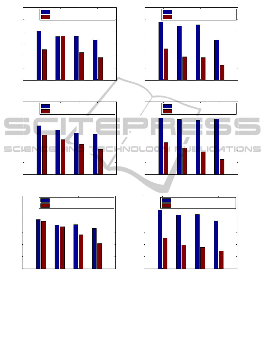
Figure 7: Training error rate comparing concatenation features and average of Fourier powers. In each ﬁgure, different EEG

channels are used. Compared with these features, concatenation features has lower error rate than average of Fourier powers,

especially in parietal and occipital areas.

Condition 2 in all time epochs. Secondly, with 1 s

epoch, ACC in Condition 2 is higher in all numbers

of features and it shows +0.06 when nu = 40.

4.3 Concatenation Method Vs.

Averaging of Signals

Finally, we compare the frequency power of a con-

catenated signal with that of the signals which are

used in concatenation. The average of Fourier pow-

ers of these signals is deﬁned as

( f ) =

NumChannel

∑

channel

(ξ

( f,channel),

(13)

where channel and NumChannel represents each

channel and total number of channels of each group,

respectively. This feature is compared with the con-

NCTA 2011 - International Conference on Neural Computation Theory and Applications

450

catenation feature ξ

to prove the effectiveness of the

concatenation method.

For comparison, SSVEP is classiﬁed with LDA

classiﬁcation with only ξ

or only ξ

. There are two

kinds of stimulus frequencies as parameters (10 and

13.33 Hz). Fig. 7 shows learning error rate in those

cases. One can observe on this ﬁgure that error rates

with concatenation features are systematically lower

than those with averaged Fourier powers.

5 DISCUSSIONS

With the concatenation method, we can obtain not

only higher frequency resolution but also higher peak

of Fourier power at the stimulus frequency. There-

fore, it may work effectively in the situation where

high temporal resolution of SSVEP detection is re-

quired. This method only requires signals concatena-

tion, consequently, it is not computationally demand-

ing, and can be used in real time processing. It re-

duces the patients’ stress when using SSVEP-BCI.

The patients are not required to focus for more than

one second, as evidenced by the 0.86 classiﬁcation

accuracy with 1 s epoch (Table 2).

In our future works, we intend to conﬁrm effects

of concatenating points with artiﬁcial signals, and in

addition to EEG signals. Moreover, using a larger

number of EEG channels could allow us to go down

to even shorter EEG epochs. One of the unsolved

problems is that each EEG epoch has different phase

and amplitudes at their borders. Therefore, the cy-

cles in each epoch do not match perfectly, which most

probably reduces the SSVEP peaks in the Fourier

spectrum. Improved algorithms for windowing EEG

epochs, and for matching their phase differences, are

to be developed.

6 CONCLUSIONS

A concatenation method is proposed to improve the

frequency resolution of Fourier spectrum when using

short EEG epochs. It successfully detected SSVEP

response by concatenating EEG epochs in the time

domain, down to 1 s windows. Classiﬁcation tests on

EEG data proved that concatenation method works

better than the averaging of Fourier spectrums com-

puted from the EEG epochs.

REFERENCES

Bashashati, A., Fatourechi, M., and Ward, R. K. (2007).

A survey of signal processing algorithms in brain-

computer interfaces based on electrical brain signals.

J. Neural Engineering, 4:R32–R57.

Bin, G., Gao, X., Yan, Z., Hong, B., and Gao, S. (2009). An

online multi-channel ssvep-based brain-computer in-

terface using a canonical correlation analysis method.

J. Neural Engineering, 6(4):046002.

Birbaumer, N. (2006). Breaking the silence: brain-

computer interfaces (bci) for communication and mo-

tor control. Psychophysiology, 43:517–532.

Dauwels, J., Vialatte, F.-B., Musha, T., and Cichocki, A.

(2010). A comparative study of synchrony measures

for the early diagnosis of alzheimer’s disease based on

eeg. NeuroImage, 49:668–693.

Dreyfus, G. (2005). Neural networks: methodology and

applications. Springer-Verlag.

Huang, N. E., Shen, Z., Long, S. R., Wu, M. C., Shih,

H. H., Zheng, Q., Yen, N.-C., Tung, C. C., and Liu,

H. H. (1998). The empirical mode decomposition and

hilbert spectrum from nonlinear and non-stationary

time series analysis. In R. Soc. Lond. A, volume 454,

pages 903–995.

Kawabata, N. (1973). A non-stationary analysis of the elec-

troencephalogram. IEEE Trans Biomed Eng, 20:444–

452.

Lotte, F., Cogedo, M., Lecuyer, A., Lamarche, F., and Ar-

naldi, B. (2007). A review of classiﬁcation algorithms

for eeg-based brain-computer interfaces. J. Neural

Engineering, 4:R1–R13.

Nunez, P. L., Srinivasan, R., Westdorp, A. F., Wijesinghe,

R. S., Tucker, D. M., Silberstein, R. B., and Cadusch,

P. J. (1997). Eeg coherency: l: statistics, refer-

ence electrode, volume conduction, laplacians, cor-

tical imaging, and interpretation at multiple scales.

Electroencephalography and Clinical Neurophysiol-

ogy, 103:499–515.

Quiroga, R., Sakowitz, O., Bas¸ar, E., and Sch¨urmann, M.

(2001). Wavelet transform in the analysis of the fre-

quency composition of evoked potentials. Brain Re-

search Protocols, 8:16–24.

Sanei, S. and Chambers, J. A. (2007). EEG signal process-

ing. Wiley, Lodon.

Vialatte, F., Sol´e-Casals, J., and Cichocki, A. (2008). Eeg

windowed statistical wavelet scoring for evaluation

and discrimination of muscular artifacts. Physiolog-

ical Measurements, 29(12):1435–1452.

Vialatte, F.-B., Maurice, M., Dauwels, J., and Cichocki, A.

(2010). Steady-state visually evoked potentials: fo-

cus on essential paradigms and future perspectives.

Progress in Neurobiology, 90:418–438.

CONCATENATION METHOD FOR HIGH-TEMPORAL RESOLUTION SSVEP-BCI

451

APPENDIX

Since y is deﬁned as (1), Fourier transform of y is

expressed as

Y(e

jω

) =

MN−1

∑

t=0

y[t]e

− jωt

N−1

∑

t=0

[t]e

− jωt

2N−1

∑

t=N

[t − N]e

− jωt

+... +

MN−1

∑

t=(M−1)N

[t − (M− 1)N]e

− jωt

∑

i=1

iN−1

∑

t=(i−1)N

[t − (i− 1)N]e

− jωt

. (14)

It also can be expressed as

Y(e

2π j f

) =

∑

i=1

iN−1

∑

t=(i−1)N

[t − (i− 1)N]e

−2π j ft

, (15)

using ω = 2π f. Furthermore, if the same signals are

concatenated (in the case of y

same

= x

= ... = x

= x, (16)

then, (15) becomes

Y(e

2π j f

) =

∑

i=1

iN−1

∑

t=(i−1)N

x[t − (i− 1)N]e

−2π j ft

. (17)

Under this condition, the constant interval depending

on the time epoch is in the case of

k = mM (m∈N), (18)

then, (19) becomes

f =

mML

. (19)

In the case of this condition,

−2π j ft

= e

−2π j f(t+nN)

(n = ... − 2,−1,0, 1,2,...)

(20)

then, (17) becomes

Y(e

2π j f

) = M

N−1

∑

t=0

x[t]e

−2π j ft

. (21)

Therefore, if (16) and (18), Fourier spectrum is M

times higher than that of an EEG signal and it has

same power distribution with each signal. Consider-

ing time epochs of 1 s, 2 s, and 5 s in Fig. 4, the

emphasized frequencies are expressed as

f =







m if L = N (1s epoch)

m/2 i f L = 2N (2sepoch)

m/5 i f L = 5N (5sepoch)

(22)

using (19).

NCTA 2011 - International Conference on Neural Computation Theory and Applications

452