
APPLICATION OF MULTIVARIATE EMPIRICAL MODE
DECOMPOSITION FOR CLEANING EYE BLINKS ARTIFACTS
FROM EEG SIGNALS
Esteve Gallego-Jutglà
1
, Jordi Solé-Casals
1
, Tomasz M. Rutkowski
2,3
and Andrzej Cichocki
2
1
Digital Technologies Group, University of Vic, Sagrada Família 7, 08500 Vic, Spain
2
LABSP, RIKEN Brain Science Institute, 2-1 Hirosawa, Saitama, 351-0106 Wako-Shi, Japan
3
Multimedia Lab, Computer Science Department & Tara Life Science Center, University of Tsukuba, Tsukuba, Japan
Keywords: EEG, mEMD, EMD, Artifacts, Eye blinks.
Abstract: Eye movements and eye blinks are present in most of the electroencephalography (EEG) recordings, making
it difficult to interpret or analyze the data. In this paper an extension of empirical mode decomposition
(EMD) is proposed in order to clean EEG data of eye blinks artifacts. This is achieved by applying two
cleaning methods to EEG simulated data. One of these methods is presented only for illustrative purposes,
whereas the second one can be applied to real EEG data. The results show that the cleaned data with both
these methods presents high correlation (
|
r
|
>0.8) with the simulated EEG clean data.
1 INTRODUCTION
Eye movements and eye blinks are undesired signals
that can introduce significant changes in the
recording of brain signals. Electric potentials due to
these artifacts can be orders of magnitude larger than
the electroencephalogram (EEG) and can propagate
across the scalp, masking and distorting brain
signals (Croft and Barry, 2000).
This paper focuses on removal of eye blinks
artifacts from EEG data using a new signal
processing technique, Multivariate Empirical Mode
Decomposition (mEMD). This technique is an
extension of the Empirical Mode Decomposition
(EMD), and provides a decomposition of the
original EEG data into several oscillatory modes
computed along multichannel data (Rehman and
Mandic, 2010). Recently it was shown that EMD is a
good method to separate eye movements from
neurophysiological signals as pointed out in
(Rutkowski et al., 2009a, Rutkowski et al., 2009b),
where results were obtained comparing the extracted
modes with the modes of the EOG.
This paper presents a new strategy for removing
eye blinks artifacts in EEG data using the mEMD
technique. In this strategy only the EEG electrodes
information is used. Two cleaning methods are
presented, and compared. The first one of these
methods is a non-realistic one, based on the use of
clean and raw EEG data, while the second one uses
only raw EEG data. These two methods are
presented in order to show that they are (almost)
equivalent and, therefore, the second method can be
used in real applications.
This paper is organized as follows. First,
methods used, including simulated data generation,
EMD and mEMD description and both cleaning
methods, are presented in Section 2. Section 3
describes the experimental results obtained with
these cleaning methods. Finally, discussion and
conclusions are presented in Section 4.
2 METHODS
EEG signals recorded on the scalp are usually highly
contaminated by various artifacts. Eye blinks are
quite often the largest ones. Typical duration of an
eye blink is 200–400 ms, and its spectral signature
spans the δ and θ range (Croft and Barry, 2000),
with most of the energy located below 5 Hz.
To eliminate eye blink artifacts, the use of
multivariate EMD (mEMD) is proposed. mEMD is
a new technique to decompose EEG data based on
EMD. mEMD decomposition is applied to simulated
EEG data and then data is cleaned using two
455
Gallego-Jutglà E., Solé-Casals J., M. Rutkowski T. and Cichocki A..
APPLICATION OF MULTIVARIATE EMPIRICAL MODE DECOMPOSITION FOR CLEANING EYE BLINKS ARTIFACTS FROM EEG SIGNALS.
DOI: 10.5220/0003722004550460
In Proceedings of the International Conference on Neural Computation Theory and Applications (Special Session on Challenges in Neuroengineering-
2011), pages 455-460
ISBN: 978-989-8425-84-3
Copyright
c
2011 SCITEPRESS (Science and Technology Publications, Lda.)
different methods. In the first method the
decompositions obtained for clean and raw EEG
data are compared in order to investigate how
artifacts affect those modes. This is not applicable in
real cases as we do not have access to clean EEG (in
fact that is what we are looking for, using cleaning
procedures). The second method is based on mEMD
of only raw EEG data, the truly accessible signals in
real applications, and is shown to be equivalent to
the first one.
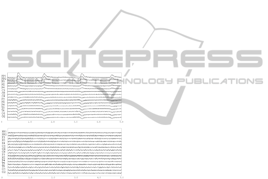
2.1 Simulated Data
In order to compare these two methods, detailed in
section 2.4, the EEG activity of 15 scalp electrodes
were simulated, 10-s of data with eye blinks (raw
EEG data) and 10-s of data without eye blinks (clean
EEG data), as shown in Figure 1. It is important to
have this raw and clean EEG data in order to
compare the results of the cleaning procedure.
Figure 1: A 5-sec portion of the simulated raw EEG time
series, with eye blinks (top image). A 5-sec portion of the
simulated clean EEG time series, without eye blinks
(bottom image).
For each realization, 4 independent cerebral
sources were simulated using the following
equation:
SourceActivit
y
=sin
2
(1)
Cerebral sources were simulated in different
frequency range (α, β, γ and μ), with consistent
location in the cortex (Kropotov, 2009) and a
sampling rate of 128 Hz. Eye blinks time series were
manually extracted using ICA decomposition on real
data. The real data was initially sampled at 1 kHz,
and before the application of ICA decomposition,
data was filtered with a band-pas filter (1 Hz- 50 Hz)
and resampled to 128 Hz with the Natural Cubic
Spline Interpolation (Congedo et al., 2002). Then,
eye blinks components of the ICA decomposition
were visually identified and extracted by its time
course and scalp topography (high gains on frontal
electrodes, small gains elsewhere) (Jung et al.,
2000).
Simulated EEG signals were derived from the
simulated cerebral sources and the extracted eye
blinks components, by multiplying by a mixing
matrix specifying the projection of each model
dipole to each sensor as sown here:
Φ=KJ+n (2)
Where vector Φ contains instantaneous scalp
electric potential differences measured at the
electrodes,J is the vector representing the impressed
current densities on the cortex (the simulated
sources), n is additive white noise, uncorrelated
withΦ, and K is the lead field matrix, which holds
the relationship between sources position and
electrodes position (Pascual-Marqui, 2002). Matrix
K was created using the low resolution brain
electromagnetic tomography software LORETA
(free publicly available academic software at http://
www.uzh.ch/keyinst/loreta.htm).
2.2 Empirical Mode Decomposition
(EMD) Applied to EEG Signals
EMD algorithm is a method designed for multiscale
decomposition and time –frequency analysis, which
can analyze nonlinear and non-stationary data
(Huang et al., 1998).
The key part of the method is the decomposition
part in which any time-series data set can be
decomposed into a finite and often small number of
Intrinsic Mode Functions (IMFs). These IMFs are
defined so as to exhibit locality in time and to
represent a single oscillatory mode. Each IMF
satisfies two basic conditions: (i) the number of
zero-crossings and the number of extrema must be
the same or differ at most by one in the whole
dataset, and (ii) at any point, the mean value of the
envelope defined by the local maxima and the
envelope defined by the local minima is zero (Huang
et al., 1998).
The EMD algorithm (Huang et al., 1998) for the
signal
can be summarized as follows.
(i) Determine the local maxima and minima of
;
NCTA 2011 - International Conference on Neural Computation Theory and Applications
456

(ii) Generate the upper and lower signal
envelope by connecting those local maxima and
minima respectively by an interpolation method;
(iii) Determine the local mean
, by
averaging the upper and lower signal envelope;
(iv) Subtract the local mean from the data:
ℎ
=
−
.
(v) If ℎ
obeys the stopping criteria, then we
define
=ℎ
as an IMF, otherwise set
=ℎ
and repeat the process from step i.
Then, the empirical mode decomposition of a
signal
can be written as:
x
t
=IMF
t
+ε
t
(3)
Where n is the number of extracted IMFs, and
the final residue ε
t
is the mean trend or a
constant.
2.3 Multivariate Empirical Mode
Decomposition (mEMD) Applied to
EEG Signals
EMD has achieved optimal results in data processing
(Diez et al. 2009, Molla et al., 2010). However, this
method presents several shortcomings in
multichannel datasets. The IMFs from different time
series do not necessarily correspond to the same
frequency, and different time series may end up
having a different number of IMFs. For
computational purpose, it is difficult to match the
different obtained IMFs from different channels
(Mutlu and Aviyente, 2011).
To solve these shortcomings, an extension of
EMD to mEMD is required. In this approach the
local mean is computed by tanking an average of
upper and lower envelopes, which in turn are
obtained by interpolating between the local maxima
and minima. However, in general, for multivariate
signals, the local maxima and minima may not be
defined directly. To deal with these problems
multiple n-dimensional envelopes are generated by
taking signal projections along different direction in
n-dimensional spaces (Rehman and Mandic, 2010).
mEMD is the technique used in this paper to
compute all the decompositions.
The algorithm (Rehman and Mandic, 2010) can
be summarized as follows.
(i) Choose a suitable pointset for sampling on an
−1
sphere (this
−1
sphere resides in an
dimensional Euclidean coordinate system).
(ii) Calculate the projection, p
t
, of the
input signal v
t
along the direction vector, x
for all k giving p
t
.
(iii) Find the time instants t
corresponding to
the maxima of the set of projected
signalsp
t
.
(iv) Interpolate t
,vt
to obtain
multivariate envelope curvese
t
.
(v) For a set of K direction vectors, the mean of
the envelope curves is calculated as
t
=
1K
⁄∑
e
t
(vi) Extract the detail
using
=
−
. If the detail
fulfills the stopping criteria
for a multivariate IMF, apply the above procedure
to
−
, otherwise apply it to
.
Then, the mEMD of a signal x
can be written
as detailed in equation 3. An example of the
application of mEMD to 5 seconds of EEG time
series with eye blinks is shown in Figure 2.
Figure 2: mEMD of 5-sec portion of the simulated raw
EEG time series (i.e. with eye blinks) at sensor FP1. The
original time series is presented in the first line (Sen). A
total of 10 IMFs are obtained for this signal.
2.4 mEMD Cleaning Procedure
2.4.1 Cleaning Method 1
The first method is based on the comparison of IMFs
obtained from the multivariate empirical mode
decomposition in the two data sets (raw data and
clean data). The key idea is to decompose each data
set and determine the similarity between modes by
means of correlation coefficients. As the only
difference between these two data sets is the
presence/absence of eye blinks, the cleaning
procedure will be focused on eliminating the modes
that are not similar in both cases, meaning that these
modes are those that appear due to eye blinks.
Therefore, the correlation between IMF of the
EEG data with eye blinks was computed with the
corresponding IMF pair of EEG data without eye
APPLICATION OF MULTIVARIATE EMPIRICAL MODE DECOMPOSITION FOR CLEANING EYE BLINKS
ARTIFACTS FROM EEG SIGNALS
457

blinks. IMFs that presented a low correlation
(
|
r
|
<0.8) were eliminated from the data before
reconstruction. This analysis was performed for each
one of the 15 electrodes existing in the dataset.
2.4.2 Cleaning Method 2
In real world applications raw data will be the only
available data. Therefore, no comparison can be
made between the mEMD decomposition and any
reference (for example, the one obtained applying
mEMD to the same cleaned data, as in the previous
case). This is why a second procedure is proposed in
order to remove eye blinks from the data.
Here the key idea is to consider that if a mode
appears in (most of) all the electrodes, this mode
cannot be due to neurological activity and therefore
it’s considered as an artifact. Note that now the only
data used is the raw EEG data (the only available
data in real applications), and common modes are
sought in the mEMD decomposition of this data.
mEMD cleaning method 2 can be summarized as
it follows:
(i) Apply mEMD to raw EEG data (EEG with
eye blinks), in order to obtain oscillatory modes of
the multivariate data.
(ii) Construct a matrix containing the same mode
of all the channels. Therefore the total number of
matrices will be equal to the number of modes we
obtained.
(iii) Calculate the correlation matrix of each one
of these previous matrices.
(iv) Calculate the mean correlation of each
channel for each mode, obtaining a vector that
contains the degree of communality of each mode
(i.e. a measure of how this mode is present in all the
electrodes). Normalize this vector in order to have
values between 0 and 1.
(v) Threshold the previous vector in order to find
which of these modes is common within all the
channels. Modes with high correlation (
|
r
|
>0.8)
are eliminated
(vi) Reconstruct clean signals without taking into
account the eliminated modes
3 RESULTS
In order to compare the performance of each
cleaning procedure, we compute the correlation
between signals at each electrode of the cleaned data
(using cleaning method 1 or cleaning method 2) and
simulated clean EEG data (EEG data without eye
blinks). The power spectra were also computed in
order to compare the differences in the frequency
domain.
Table 1 shows the eliminated modes with each
cleaning method. Reconstructed signals were
computed without those IMFs.
Table 1: Eliminated IMFs for each cleaning method.
Sensors Eliminated IMFs
Method 1
Fz and O1 4, 5, 6, 7, 8 and 9
F4, C3, P4, P3,
T5, T6 and O2
4, 5, 6, 7, 8, 9 and 10
F3 and C4
4, 5, 6, 7, 8, 9 and ε
t
FP1, FP2, Cz
and Pz
4, 5, 6, 7, 8, 9, 10 and ε
t
Method 2
All sensors
4,5,6,7,8,9, 10 and ε
t
As can be seen in Table 1, results are very
similar, differing only on the final IMF 10 and the
residue
ε
t
. For the cleaning method 1 some
sensors kept those modes and some sensors
eliminate them, whereas cleaning method 2
eliminated all IMF form IMF 4 to IMF 10 and the
residue
ε
t
.
The correlation between reconstructed data with
method 1 and method 2 and the simulated clean
EEG signal (without eye blinks) is presented in
Figure 3. This figure also shows (blue bars) the
correlation between the original raw EEG data (with
eye blinks) and the clean EEG data (without eye
blinks)
Clearly it can be seen that eye blinks disturb
EEG data in such a way that correlation between raw
EEG and clean EEG is very low in all the electrodes
(blue bars in Figure 3), and especially in frontal
electrodes FP1 and FP2, as they are close to eyes.
Using cleaning procedures to eliminate eye blinks
allows us to recover an approximation of clean EEG
data, and this can be observed in the correlation of
data between clean EEG and cleaned EEG data at
each electrode, whatever method is used (green and
brown bars in Figure 3).
Initial correlation of data with eye blinks is
highly improved with both two cleaning procedures,
with correlation values
|
r
|
>0.8. Despite no
significant differences between the two cleaning
methods, cleaning method 2 always presents higher
correlation than cleaning method 1.
The power spectra of the frontal electrodes (FP1 and
FP2) are presented in Figure 4. Results show that the
simulated EEG data with eye blinks (blue line)
presents more power in the low frequencies, whereas
no such power appears in the power spectra of the
EEG data without eye blinks (black line). Even if the
reconstructed
signal with method 2 (red line)
NCTA 2011 - International Conference on Neural Computation Theory and Applications
458
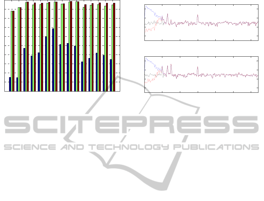
Figure 3: Correlations, at each sensor, of the simulated
clean EEG with raw EEG data (blue), cleaned EEG data
with cleaning method 1 (green) and cleaned EEG data
with cleaning method 2 (red).
presents less power spectra in the low frequencies
than the clean EEG data, its shape is more similar to
the (original) clean EEG data than the raw data, and
no differences can be observed in the higher
frequencies (α, β and γ range) between them.
4 DISCUSSION AND
CONCLUSIONS
In this paper a new procedure for cleaning eye blink
artifacts in EEG data is presented. This new method
is based on a novel EEG decomposing technique,
which allows flexible signal decomposition of the
original time series in different oscillatory modes.
The so-obtained components from each EEG
channel have been analyzed using two different
strategies. In method 1, the obtained IMFs have been
compared with the IMFs from artifacts-clean EEG
data and those that presented low correlation
havebeen eliminated in the reconstruction process.
On the other hand, in method 2 the obtained IMFs of
the raw EEG data of all electrodes have been
compared among themselves, and those that are
present in all the electrodes have been eliminated in
the reconstruction process. Resulting reconstruction
in both methods allowed us to separate eye blinks
artifacts from brain activity.
The two methods presented in this article
achieved a suppression of the eye blinks artifacts.
However, method 1 is based on the comparison of
raw EEG data with clean EEG data (that is not
available in real scenarios), therefore is not a useful
method
and was presented here for illustrative
Figure 4: Power spectra of the frontal electrodes FP1
(upper image) and FP2 (bottom image). In blue, the power
spectra of the simulated raw EEG data (with eye blinks);
in black, the power spectra of the simulated clean EEG
data (without eye blinks); and in red, the power spectra of
the reconstructed data with cleaning method 2.
purposes. On the other hand, method 2 uses only raw
EEG data and in our experiments has been shown to
be (almost) equivalent to method 1, giving the same
or better results in cleaning eye blinks artifacts.
The eliminated modes presented in Table 1
correspond to low frequency oscillation. These
results are consistent with previous knowledge of
eye blinks artifacts, in which the artifact interference
is found in the low frequencies.
Finally, results in Figure 4 show that power
spectra due to the eye blinks artifacts in δ and θ
bands are clearly suppressed, whereas the power in
the higher frequency range (α, β and γ bands) do not
present significant differences.
These results point out that the use of mEMD to
correct eye blinks may be a good procedure for EEG
signal preprocessing, a necessary step to be taken
before any kind of EEG signal analysis.
Future work will include the comparison of this
method with ICA-based cleaning procedures (Solé-
Casals et al., 2010), or Wavelet-based cleaning
procedures (Krishnaveni et al., 2006, Vialatte et al.,
2008), and optimization of the computational load in
order to obtain a real-time system.
ACKNOWLEDGEMENTS
The authors would like to express their gratitude to
the reviewers for their valuable suggestions. This
work has been partially supported by the Fundación
Alicia Koplowitz to Dr. Jordi Solé-Casals, and by the
FP1 FP2 F3 FZ F4 C3 CZ C4 P3 PZ P4 T5 T6 O1 O2
0
0.1
0.2
0.3
0.4
0.5
0.6
0.7
0.8
0.9
1
0 10 20 30 40 50 60
-6
-4
-2
0
Sensor FP1
log(magnitude)
[Frequency]
0 10 20 30 40 50 60
-6
-4
-2
0
Sensor FP2
log(magnitude)
[Frequency]
APPLICATION OF MULTIVARIATE EMPIRICAL MODE DECOMPOSITION FOR CLEANING EYE BLINKS
ARTIFACTS FROM EEG SIGNALS
459

University of Vic under de grant R0904.
REFERENCES
Congedo, M., Ozen, C., Sherlin, L. (2002). Notes on EEG
resampling by natural cubic spline interpolation.
Journal of Neurotherapy, 6(4).
Croft, R. J., Barry, R. J., (2000). Removal of ocular
artefact form the EEG: a review. Neurophysiol
Clin,30, 5-19.
Diez, P. F., Mut, V., Laciar, E., Torres, A., Avilla, E.
(2009). Application of the Empirical Mode
Decomposition to the Extraction of Features form
EEG signals for Mental Task Classification. 31
st
Annual International Conference of the IEEE EMBS.
2579-2582.
Huang, N. E., Shen, Z., Long, S. R., Wu, M. C., Shih, H.
H., Zheng, Q., Yen, N. C., Tung, C. C., Liu, H. H.
(1998). The empirical mode decomposition and the
Hilbert spectrum for nonlinear and non-stationary time
series analysis. Proc. R. Soc. Lond., 495, 2317-2345.
Jung, T. P., Makeig, S., Westerfield, M., Townsend, J.,
Courchesne, E., Sejnowski, T. J. (2000). Removal of
eye artifacts from visual event-related potentials in
normal and clinical subjects. Clinical
Neurophysiology, 111, 1745-1758.
Kropotov, J. D., (2009). Quantitative EEG Event-Related
Potentials and Neurotherapy. (1st ed.). San Diego:
Academic Press.
Krishnaveni, V., Jayaraman, S., Aravind, S.,
Hariharasudhan, V., Ramadoss, K. (2006). Automatic
Identification and Removal of Ocular Artifacts from
EEG using Wavelet Transform. Measurement Science
Review, Vol. 6, Sec. 2, No. 4.
Molla, K. I., Tanaka, T., Rutkowski, T. M., Cichocki, A.,
(2010). Separation of EOG artifacts from EEG singals
using bivariate EMD. Acoustics Speech and Signal
Processing (ICASSP), 2010 IEEE Interational
Conference On. 562-565.
Mutlu, A. Y., Aviyente, S. (2011). Mutivariate Empirical
Mode Decomposition for Quantifying Multivariate
Phase Synchronization. EURASIP Jounal on Advances
in Signal Processing. Article ID 615717.
Pascual-Marqui, R. D. (2002). Standardized low resolution
brain electromagnetic tomography (sLORETA):
technical details. Methods Find. Exp. Clin.
Pharmacol.,24D, 5-12.
Rehman, N., Mandic, D. P., (2010). Multivariate empirical
mode decomposition. Proc. R. Soc. A. 466, 1291-
1302.
Rutkowski, T. M., Cichocki, A., Tanaka, T., Mandic, D.
P., Cao, J., Ralescu, A. L., (2009a). Multichannel
spectral pattern separation – An EEG processing
application. 2009 IEEE International Conference on
Acoustics, Speech and Signal Processing.
Rutkowski, T. M., Cichocki, A., Tanaka, T., Ralescu, A.
L., Mandic, D. P., (2009b). ICONIP’08 Proceedings
of the 15
th
international conference of Advances in
neuro-information processing. Vol Part I.
Solé-Casals, J., Vialatte, F. B., Pantel, J., Prvulovic, D.,
Haenschel, C., Cichocki, A.: ICA Cleaning Procedure
for EEG Signals Analysis - Application to Alzheimer's
Disease Detection. BIOSIGNALS 2010: 484-489
Vialatte, F. B., Solé-Casals, J., Cichocki, A. (2008). EEG
windowed statistical wavelet scoring for evaluation
and discrimination of muscular artifacts. Physiol.
Meas. 29 1435–1452.
NCTA 2011 - International Conference on Neural Computation Theory and Applications
460
