INFERENTIAL MINING FOR RECONSTRUCTION OF 3D CELL

STRUCTURES IN ATOMIC FORCE MICROSCOPY IMAGING

Mario d’Acunto

, Stefano Berrettini

, Serena Danti

, Michele Lisanti

, Mario Petrini

Andrea Pietrabissa

and Ovidio Salvetti

Istituto di Scienze e Tecnologia dell’Informazione, ISTI-CNR, via Moruzzi 1, I-56124, Pisa, Italy

Dept. of Neuroscience, University of Pisa, via Roma 55, 56126, Pisa, Italy

Dept. of Orthopedics &Traumatology, University of Pisa, via Paradisa 2, 56124, Pisa, Italy

Dept. of Oncology & Transplants, University of Pisa, via Roma 55, 56126, Pisa, Italy

Dept. of Surgical Sciences, IRCCS Policlinico San Matteo, University of Pavia, 27100 Pavia, Italy

Keywords: Atomic Force Microscopy imaging, 3D cell reconstruction, Bayesian single frame high-resolution.

Abstract: Atomic Force Microscopy (AFM) is a fundamental tool for the investigation of a wide range of mechanical

properties on nanoscale due to the contact interaction between the AFM tip and the sample surface. The

focus of this paper is on an algorithm for the reconstruction of 3D stem-differentiated cell structures

extracted by typical 2D surface AFM images. The AFM images resolution is limited by the tip-sample

convolution due to the combined geometry of the probe tip and the pattern configuration of the sample. This

limited resolution limits the accuracy of the correspondent 3D image. To drop unwanted effects, we adopt

an inferential method for pre-processing single frame AFM image (low resolution image) building its super-

resolution version. Therefore the 3D reconstruction is made on animal cells using a Markov Random Field

approach for augmented voxels. The 3D reconstruction should improve unambiguous identification of cells

structures. The computation method is fast and can be applied both to multi- and to single-frame images.

1 INTRODUCTION

In this paper, we adopt an inferential procedure

providing a high-resolution algorithm for the single-

image AFM raw data and then the construction of a

3D routine for the improved resolution images.

When applied to cell populations, the 3D

reconstruction, as developed in this paper, is a useful

tool for the recognition of cell patterns and organs

and it could be used for a fast in situ analysis for

biologists and biomedical scientists.

In the last two decades, AFM has been

developed well beyond the topographic imaging

tool. It has become an important instrument for

manipulation and material property characterizations

at the nanometer scale. The precision of positioning

has always been the key driver for AFM technology

and scanning probe microscopy in general.

Nevertheless, uncontrolled hardware drift, such as

piezo creep and thermal drift, can cause image

distortion and limiting resolution. Some solutions

based on offline corrections (Yurov and Klimov,

1994), hardware optimization (Hug et al., 1992;

Altmann et al., 2000; Beyder et al., 2006), image

based real-time compensation (Clayton and Devasia,

2005), or image-based adaptive control has been

proposed (Belikov et al., 2008; D’Acunto and

Salvetti, 2011). An AFM probe tip measures the

topography of a surface by looking the vertical

deflection of a cantilever and then associating a z-

height value to the correspondent vertical deflection.

The resulting image is obtained plotting the function

=f(x

), for any couple (x

) of the sample

surface. The focus of this paper is to build a method

for a 3D reconstruction after the acquired AFM

image is processed in order to obtain its High-

Resolution (HR) representation.

HR methods are techniques that enhance the

resolution of an imaging system. In optical based

imaging, HR techniques break the diffraction-limit,

analogously, HR methods can improve the

resolution of digital imaging sensors. HR techniques

can be divided in two categories, single-frame or

multiple-frame, respectively. Multiple-frame HR use

the sub-pixel shifts between multiple low resolution

images of the same scene. On the contrary, single

348

D’Acunto M., Berrettini S., Danti S., Lisanti M., Petrini M., Pietrabissa A. and Salvetti O..

INFERENTIAL MINING FOR RECONSTRUCTION OF 3D CELL STRUCTURES IN ATOMIC FORCE MICROSCOPY IMAGING.

DOI: 10.5220/0003685503400345

In Proceedings of the International Conference on Knowledge Discovery and Information Retrieval (KDIR-2011), pages 340-345

ISBN: 978-989-8425-79-9

 2011 SCITEPRESS (Science and Technology Publications, Lda.)

frame HR methods attempt to magnify the image

without introducing blur. These last methods use

other parts of the low resolution images to make an

extimation on what the high resolution images

should look like. AFM imaging requires to work

using a single-frame approach: given a single image

of sample scanned at low resolution, return the

image that is mostly likely to be generated from a

noiseless high resolution scan of the same sample

portion. After HR equilavent image is reached, 3D

recostruction is made possible using a Markov

Random Field (MRF) approach. In a MRF method

we consider a couple (h

, N), where a stochastic

process is indexed by an augmented voxel h

for

which, for every couple (x,y) of the 2D image, any

augmented voxel depends only on its immediate

neighbours of the N set, where N is a parameter

space. The choice of N depends by the system

variables conditional probability distributions, where

system variables provide the basic tool for modelling

spatial continuity.

We apply our method to cells derived by stem

primitive cells and differentiated in osteocytes or

adipocytes, or fibroblast. Any differentiated stem

cell develops specific organs and functions, and

recognition such organs is not a trivial question. The

3D reconstruction is useful when does not lose

information of the primitive image and gives the

possibility to identify unambiguous such specific

organs.

2 INFERENTIAL GENERATIVE

MODEL

Despite the AFM ability to reach high spatial

resolution, the acquired surface topography image

can sometimes not correspond to the real surface

features due to the effect of the instrument on the

object producing artefacts. These artefacts can be

generally taken into consideration while

qualitatively interpreting the AFM results. However,

3D reconstruction tools require quantitative

estimation and reconstruction of sample true

geometry. During scanning, two major AFM

artefacts can appear: a profile broadening effect due

to the tip-sample convolution and the height

lowering effect due to the elastic deformation of

studied samples.

The first effect can be schematised as follows:

the tip moving across an object surface can be

approximated by a sphere of radius R moving along

a sphere of radius r surface, i.e., the tip describes arc

of radius R+r. The lateral dimension of the surface

objects is r

=2(R

⋅

1/2

and the relative height of the

object

z=r[1-(1-(r

/(R+r))

]

(1)

The minimum separation between two asperities or

local pattern that can be detected is d= (8RΔz)

1/2

, that

is also the lateral resolution.

Before to build the 3D structures, the source

images are processed in order to improve their

resolution. To do this operation, we adopt a

Bayesian method. Hardie et al (Hardie et al, 1997)

demonstrated that low-resolution images can be

updated using super-resolution image estimate, and

that this improves a Maximum a Posteriori (MAP)

super-resolution image estimate. Pickup et al.

(Pickup et al., 2009) used a similar joint MAP

approach to learn more general geometric patterns,

configuring the correspondent super-resolution

images and valuing the prior parameters

simultaneously. Another remarkable result for the

inferential super-resolution has been reached by

Tipping and Bishop (Tipping and Bishop, 2003),

they used a Maximum Likelihood (ML) point

estimate of the image parameters found by

integrating the high-resolution image out the

registration problem and optimising the marginal

probability of the observed low-resolution images

directly.

We follow a generative model based on an idea

as proposed by Torres-Mendez et al. (Torres-

Mendez et al., 2007) carried out from single-frame

methods. The basic idea can be summarized as

follows: given a Low Resolution (LR) image α of

size h

×w

pixels, we want to estimate the

correspondent HR image ω of size h

×w

, with

equal or greater size of the input image α. From α,

we must generate L images of smaller size (scaled),

that we can call observable images l, with l=0…L.

Any point in the LR image is considered as a node in

a Markovian process, and a possible neighbourhood

node in the HR image is defined by a pairwise

potential. If we denote x

as a set of hidden nodes in

the output ω, and the y

as the observable nodes in α

image, and defining the pairwise potential between

the variables x

, and x

, by

and the local evidence

potential associated with the variables x

and y

, the joint probability correspondent to the

Markovian process can be written as

()

(

)

()

iji

yxxx

yxP ,,

∏∏

= Φ

(2)

where Z is a normalization constant. Our problem

consists to maximize P(x,y), maximization that

corresponds to find the most likely state for all

hidden nodes x

, given all the node y

. To remove

INFERENTIAL MINING FOR RECONSTRUCTION OF 3D CELL STRUCTURES IN ATOMIC FORCE

MICROSCOPY IMAGING

349

ambiguities, we decide to assign high compatibility

between neighbouring pixels that have similar

intensity values and low compatibility between

neighbouring pixels that present drastic changes in

their intensity values. The value of any single pixel

in HR ω image is obtained estimating the maximum

a posteriori (MAP) solution associated to the MRF

model as given by eq. (2)

(

)

αωω

MAP

maxarg=

(3)

where

(

)

(

)

()

iji

yxxx

PPP

∏∏

∝∝

ωωααω

(4)

Being the conditional probabilities impossible to

be exactly computed, because it is impossible to

represent all the possible combinations between

pixels, we adopt a Markov Chain Monte Carlo

(MCMC) method to approximate the best solution of

(3). The HR images so obtained are still 2D

representation of the acquired AFM images. The

correspondent 3D reconstruction is discussed in the

next section

3 3D RECONSTRUCTION

MODEL

The typical visual rendering of AFM images

describes the recorded structures assessing a gray

intensity (o colour intensity) to the z=f(x,y) measured

value. This is not properly a 3D reconstruction. 3D

reconstruction is possible in tomography-based

techniques thanks to the multi-acquisition of images

at different angles and then recollected in a unique

image via Radon anti-transformation, for example.

When the source is composed by a unique image,

the 3D reconstruction is rather complicated, and the

possibility to introduce artefacts or unwanted effects

is high. Our method is based on learning a statistical

model of the local relationship between the observed

range data and the variations in the intensity image

and uses this model to compute unknown depth

values. The intensity of any point is supposed to be a

Markov process. Unknown depth values are then

inferred by using the statistics of the observed range

data to determine the behaviour of the Markov

process. The presence of intensity where range data

is being inferred is crucial since intensity provides

knowledge of surface smoothness and variations in

depth. The advantage of our approach is to carry out

knowledge directly from the observed data, without

to introduce constraints that could be inapplicable to

particular environments. Although if our method

seem to be very close to a traditional shape-from-

shading method (where depth inference from

variations in surface shading), the substantial

difference is in the inferential engine that connects

the final 3D reconstruction to a suitable processing

of original data.

3.1 Reconstruction Methodology

Our goal is to infer a dense range map from an

intensity image and a very sparse initial range data.

The inference on range data is solved using a

sampling on the intensity at each point considered as

a product of a Markovian process. Unknown range

data is then inferred by using the statistics of the

observed range data to determine the behaviour of

the Markovian process. In our approach, there some

critical aspects, for example, the knowledge

extracted from smooth intensity variation could

generate artefacts, or again, the right weight of a

variation in depth.

The starting point is the development of a set of

augmented voxels V that contain intensity, edge

(from the intensity range) and range information. It

should be mentioned that the intensity can be

considered both for gray scales or colour images,

and that the range information includes portion of

ranges a priori unknown). Let us introduce Ω as the

area of unknown range that corresponds to the

region to be filled. Following Torres-Mendez et al.

(Torres-Mendes et al, 2007), we base our

reconstruction method on the amount of reliable

information surrounding the augmented voxel whose

depth value is to be estimated, and also on the edge

information. Thus, for each augmented voxel V

count the number of neighbour voxels with already

assigned range and intensity. A general criterion is

to start by reconstructing those augmented voxels

which have more of their neighbour voxels already

filled, leaving to the end those with an edge passing

through them. After a depth value is estimated, we

update each of its neighbours by adding 1 to their

own neighbour counters. The next step is to proceed

to the subsequent groups of augmented voxels to

synthesise until no more augmented voxels in Ω

exists.

Formally, an augmented voxel is defined as

V=(z,E,R) where z denotes the pixel intensity

directly connected to the z-height as measured by the

AFM, E is a binary matrix (1 if an edge exits, 0

otherwise) and R denotes the matrix of incomplete

pixels depth. It is possible to define a set of

KDIR 2011 - International Conference on Knowledge Discovery and Information Retrieval

350

augmented voxels that lie on each ray that intersects

each pixel of the input image z, thus giving us a

registered range image R and intensity image z. Let

=(x,y): 1≤x,y≤m denote the m integer lattice , then

z={z

x,y

}, (x,y)∈h

, denotes the gray levels of the

input image, and r={R

x,y

}, denotes the depth values.

Than we model the V set as a Markov Random

Field. Within the Markov Random Field picture, z

and R must be considered random variables. Let us

introduce a neighbourhood system, defined as

N={N

x,y

∈h

}, where N

x,y

⊂h

denotes the neighbours

of (x,y).

A Markov Random Field over (h

, N) is a

stochastic process indexed by h

for which, for

every couple (x,y) any augmented voxel depends

only on its immediate neighbours. The choice of N

together with the conditional probability distribution

of P(z) and P(R) provides the basic tool for

modelling spatial continuity. Therefore, the N

x,y

set

is modelled on the acquisition data matrix that is a

square mask of size n×n centered at the augmented

voxel location (x,y). The calculation of the

conditional probabilities in an explicit form is an

infeasible task since we cannot efficiently represent

or determine all the possible combinations between

augmented voxels with its associated neighbours. To

do this calculation we can invoke the Gibbs

sampling, for example, and average a depth value

from the augmented voxel V

x,y

with neighbours N

x,y

by selecting range value from the augmented

resembles the region being filled voxel whose

neighbours N

k,l

most resembles the region being

filled in

lkyx

Alk

opt

NNN

),(

minarg

−=

∈

(5)

where A={A

k,l

⊂N} is the set of local neighborhood,

in which the center voxel has already assigned a

depth value, such that 1≤[(k-x)

+(l-y)

]

1/2

≤d. For

each successive augmented voxel, N

opt

as given by

Eq. (5) approximates the maximum a posteriori

estimate. The distance || ⋅ || is defined as the

weighted sum of squared differences over the partial

data in two neighbourhoods. The weights are choice

applying 2D Gaussian kernel to each

neighbourhood, such that those voxels near the

center are given more weight than those at the edge

of the window.

4 RESULTS

In this section, we present the basic results inherent

the 3D model as discussed in the past two sections.

The primitive AFM images are processed in order to

improve their quality (ranging from LR to HR) and

then the algorithm for their 3D reconstruction using

the MRF picture as given by Eq. (5) is applied.

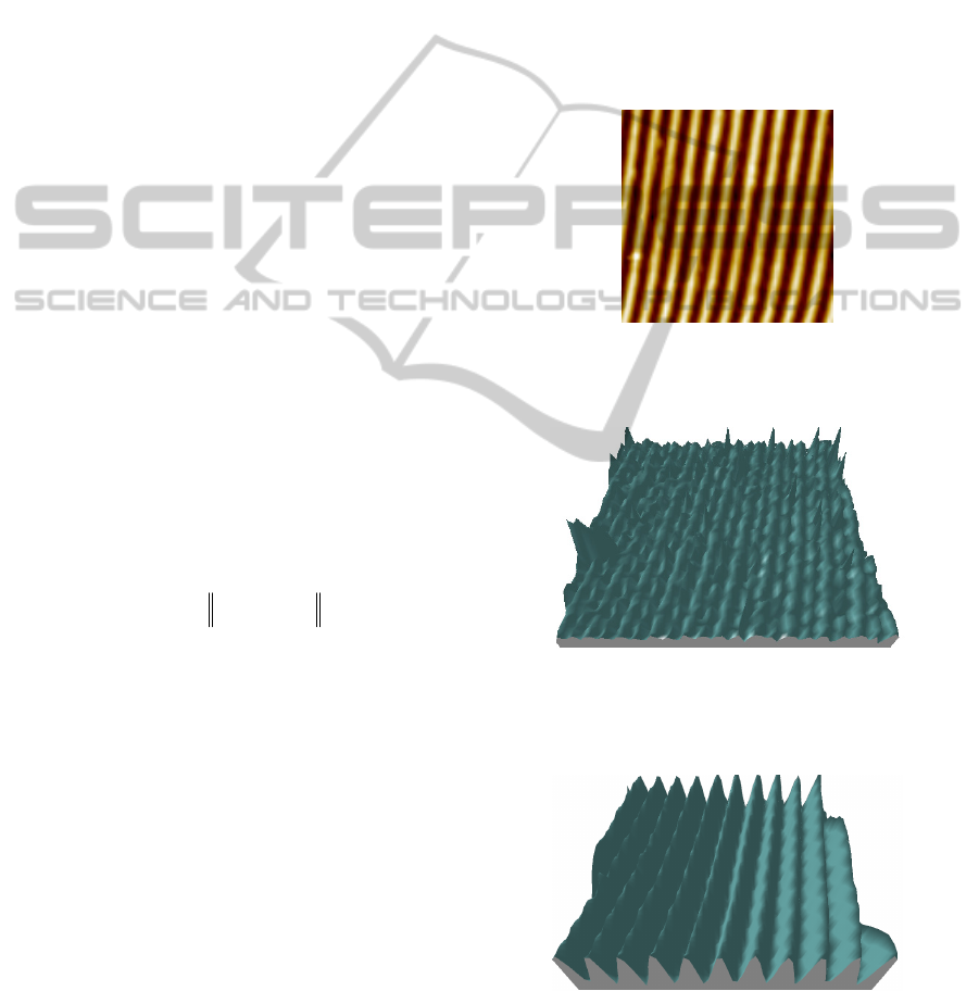
Firstly, the method is used on images of regular

lattice for AFM calibration to sample with

nanometers patterns. Figure 1 shows silicon grating,

normally used for calibration of z-height in AFM

measurements. Its accurate 3D reconstruction of the

grains is of great importance. It should be noted that

the image in figure 1 has not been pre-processed and

it presents an artefact at the bottom, while the image

in figure 3 that represents its correspondent 3D

reconstruction corrects such artefact.

Figure 1: Silicon grating used for AFM calibration of z-

height. The mounds are large 100nm and periodicity is

200nm.

Figure 2: 3D reconstruction of the image as in figure 1

without HR processing of the 2D image. Some artefacts

and topographic roughness present in the primitive 2D

image are amplified and the grating is not well resolved.

Figure 3: 3D reconstruction of the grating as in figure 1

with HR processing applied on the image as recorded by

the AFM. In this case, the artefacts are removed and the

grating presents a spatially well-resolved structure, where

mounds and valleys are clearly separated.

INFERENTIAL MINING FOR RECONSTRUCTION OF 3D CELL STRUCTURES IN ATOMIC FORCE

MICROSCOPY IMAGING

351

Now, we apply our procedure to cell images. The

cell samples are obtained in cellular cultures from

pluripotent stem cells and differentiated in

osteocytes, fibroblasts, adipocytes or others (Danti et

al. 2006).

A typical problem acquiring images on cells

using an AFM is the low resolution due large

dimensions of cells and reduced instrumental

capability to increase pixels. For example, many

commercial AFM can perform measurement with a

pixel density of 512×512 or 1024×1024 pixels.

Because some animal cells present dimensions that

needs scans on area of 100μm×100μm, this implies

that any single pixel covers approximately an area of

100nm×100nm for a pixel density of 1024×1024.

For this reason, the increasing of resolution can play

a fundamental role for the recognition of cells

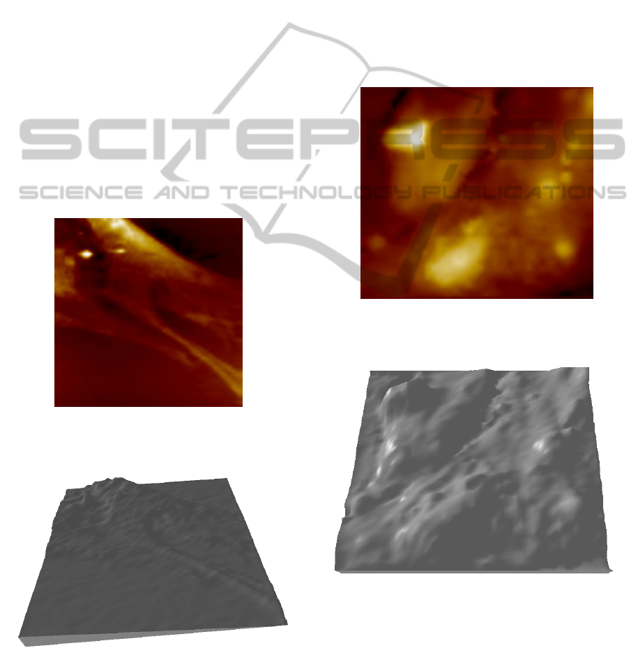
patterns or organ shapes. Figure 4 presents an image

of a large osteocyte. The primitive image is low

resolution, 512×512 pixels on an area 50μm×50μm,

after LR to HR method is applied, the 3D

reconstruction presents all the characteristics

features as in the 2D AFM image

Figure 4: AFM image of a portion of an osteocyte (real

area surface 50μm×50μm, z-height less than 5μm, density

pixel 512×512).

Figure 5: The correspondent 3D reconstruction of the

osteocyte as in figure 4.

In many cases, another problem generally found

during the imaging of cells is the identification of

specific cells in a cluster. In fact, in a cell culture,

the differentiation is often followed by meiosis, so

producing a population of cells partially overlapping

one each other. This is the case of the adipocytes

displayed in figure 6. Two nuclei are well

recognized, but it is not so for the cell edges. The 3D

reconstruction can help to identify cells dimensions

and organs in a manner that is not possible in the 2D

image and correspondent three-dimensional visual

rendering performed both with open source

(Gwyddion, http://gwyddion.net) or commercially

available programs (SPIP, http://www.imagemet.com)

Figure 6: AFM image of a cluster of adipocytes (real area

surface 50μm×50μm, z-height approximately 8μm,

density pixel 512×512).

Figure 7: 3D reconstruction of the cluster cells as in figure

6. The cells structures are well defined, it is possible to

recognize the nuclei.

5 CONCLUSIONS

Atomic Force Microscopy (AFM) is a fundamental

KDIR 2011 - International Conference on Knowledge Discovery and Information Retrieval

352

tool for the investigation of a wide range of

mechanical properties on nanoscale due to the

contact interaction between the AFM tip and the

sample surface. The information recorded with AFM

is stored and synthesized by imaging the sample

properties to be studied. The AFM topographic

images are matrices z=f(x,y), that links a z-value to

the correspondent x,y surface point. The focus of this

paper is on an algorithm for the reconstruction of 3D

structures extracted by typical 2D surface AFM

images. The AFM images resolution is limited by

the tip-sample convolution due to the combined

geometry of the probe tip, density pixels and specific

the pattern configuration of the sample. This limited

resolution reflects on the accuracy of the

correspondent 3D image. We have adopted an

inferential procedure that provides a high-resolution

algorithm for the single-image AFM raw data and

then the construction of a 3D routine for the

improved resolution images. When applied to cell

populations, the 3D reconstruction are an useful tool

for the recognition of cell pattern and organs and it

could be used for a fast in situ analysis for biologists

and biomedical scientists.

REFERENCES

Altmann S. M., Lenne P. F., Horber H., 2000. Rev. Sci.

Instrum., 72, 142-149.

Amit Y., Grenader U., Piccioni M., 1991. J. Amer. Statist.

Assoc. 86, 376-387.

Amit Y., 1994. SIAM J. Sci. Comput., 15, 207-224.

Belikov S., Shi J., Su C., 2008. American Control

conference Seattle Washington, USA, ThA08.5 (1-5).

Beyder A., Spagnoli C., Sachs F., 2006. Rev. Sci. Instrum.,

77, 1551-7.

Clayton, G. M., Devasia, S., 2005. Nanotechnology 16,

809–818.

D’Acunto M., Salvetti O., 2011, Pattern Recognition and

Image Analysis, 21, 9-19.

Danti, S., D’Acunto M., Trombi L., Berrettini S.,

Pietrabissa A., 2007. Macromolecular Bioscence, 7,

589-598.

Flores F. C., de Alecar Lotufo R., 2010. Image and Vision

Computing, 28, 1491-1514.

Gonzalez, R., Wood, R., 2008. Digital Image Processing.

Upper Saddle River, NJ, Prentice Hall.

Hardie R. C., Barnard K. J., Armstrong E. E., 1997, IEEE

Transactions on Image Processing, 6, 1621-1633.

Henn S., Witsch K., 2000. Computing, 64, 339-348.

Henn S., Witsch K., 2001. SIAM J. Sci. Comput., 23,

1077-1093.

Hug H. J., Yung T., Güntherodt H. J., 1992. Rev. Sci.

Instrum., 63, 3900-3904.

Pickup L. C., Capel D. P., Roberts S. J., Zissermann A.,

2009. The Computer Journal, 52(1), 101-113.

Tipping M. E. Bishop C. M., 2003. In Becker S. Thrun S.

and Obermeyer K. (Eds.), Advances in Neural

Information Processing Systems, 15, 1303–1310.

Torrez-Mendez L. A., Ramirez-Sosa Moran M.I., Castela

M., 2007. In Gelbuck A., Kuri Morales A. F., MICAI

2007, LNAI 2007, 640-649. Springer-Verlag Berlin

Heidelberg.

Yurov, V. Y., Klimov, A. N., 1994. Rev. Sci. Instrum.,

65(5) 1551-7.

INFERENTIAL MINING FOR RECONSTRUCTION OF 3D CELL STRUCTURES IN ATOMIC FORCE

MICROSCOPY IMAGING

353