
DECENTRALIZED NEURAL BACKSTEPPING CONTROL FOR
AN INDUSTRIAL PA10-7CE ROBOT ARM
R. Garcia-Hernandez
1
, E. N. Sanchez
2
, M. A. Llama
3
and J. A. Ruz-Hernandez
1
1
Facultad de Ingenieria, Universidad Autonoma del Carmen, Av. 56 No. 4, Cd. del Carmen, Campeche, Mexico
2
Centro de Investigacion y de Estudios Avanzados del IPN, Unidad Guadalajara, Guadalajara, Jalisco, Mexico
3
Division de Estudios de Posgrado, Instituto Tecnologico de la Laguna, Torreon, Coahuila, Mexico
Keywords:
High-order neural network, Extended Kalman filter, Backstepping, Trajectory tracking, Robot arm.
Abstract:
This paper presents a discrete-time decentralized control strategy for trajectory tracking of a seven degrees
of freedom (DOF) robot arm. A high order neural network (HONN) is used to approximate a decentralized
control law designed by the backstepping technique as applied to a block strict feedback form (BSFF). The
neural network learning is performed online by extended Kalman filter. The local controller for each joint use
only local angular position and velocity measurements. The feasibility of the proposed scheme is illustrated
via simulation.
1 INTRODUCTION
Nowadays, industrial robots have gained wide pop-
ularity as essential components in the construction
of automated systems. Reduction of manufacturing
costs, increase of productivity, improvement of prod-
uct quality standards, and the possibility of eliminat-
ing harmful of repetitive tasks for human operators
represent the main factors that have determined the
spread of the robotic technology in the manufactur-
ing industry. Industrial robots are suitable for applica-
tions where high precision, repeatability and tracking
accuracy are required.
In this context, a variety of control schemes have
been proposed in order to guarantee efficient tra-
jectory tracking and stability (Sanchez and Ricalde,
2003), (Santiba˜nez et al., 2005). Fast advance in
computational technology offers new ways for imple-
menting control algorithms within the approach of a
centralized control design.However, there is a great
challenge to obtain an efficient control for this class of
systems, due to its highly nonlinear complex dynam-
ics, the presence of strong interconnections, parame-
ters difficult to determine, and unmodeled dynamics.
Considering only the most important terms, the math-
ematical model obtained requires control algorithms
with great number of mathematical operations, which
affect the feasibility of real-time implementations.
On the other hand, within the area of control sys-
tems theory, for more than three decades, an alter-
native approach has been developed considering a
global system as a set of interconnected subsystems,
for which it is possible to design independent con-
trollers, considering only local variables to each sub-
system: the so called decentralized control (Huang
et al., 2003). Decentralized control has been applied
in robotics, mainly in cooperative multiple mobile
robots and robot manipulators, where it is natural to
consider each mobile robot or each part of the ma-
nipulator as a subsystem of the whole system. For
robot manipulators each joint and the respective link
is considered as a subsystem in order to develop local
controllers, which just consider local angular position
and angular velocity measurements, and compensate
the interconnection effects, usually assumed as dis-
turbances. The resulting controllers are easy to im-
plement for real-time applications (Liu, 1999).
In (Ni and Er, 2000), a decentralized control of
robot manipulators is developed, decoupling the dy-
namic model of the manipulator in a set of linear sub-
systems with uncertainties; simulation results for a
robot of two joints are shown. In (Karakasoglu et al.,
1993), an approach of decentralized neural identifica-
tion and control for robots manipulators is presented
using models in discrete-time. In (Safaric and Rodic,
2000), a decentralized control for robot manipulators
is reported; it is based on the estimation of each joint
dynamics, using feedforward neural networks.
In recent literature about adaptive and robust con-
trol, numerous approaches have been proposed for
82
Garcia Hernandez R., N. Sanchez E., A. Llama M. and A. Ruz-Hernandez J..
DECENTRALIZED NEURAL BACKSTEPPING CONTROL FOR AN INDUSTRIAL PA10-7CE ROBOT ARM.
DOI: 10.5220/0003684300820089
In Proceedings of the International Conference on Neural Computation Theory and Applications (NCTA-2011), pages 82-89
ISBN: 978-989-8425-84-3
Copyright
c
2011 SCITEPRESS (Science and Technology Publications, Lda.)

the design of nonlinear control systems. Among
these, adaptive backstepping constitutes a major de-
sign methodology (Krstic et al., 1995). The idea be-
hind the backstepping approach is that some appro-
priate functions of state variables are selected recur-
sively as virtual control inputs for lower dimension
subsystems of the overall system. Each backstepping
stage results in a new virtual control design from the
preceding stages; when the procedure ends, a feed-
back design for the true control input results, which
achieves the original design objective.
In this paper, the authors propose a decentral-
ized approach in order to design a suitable controller
for each subsystem. Afterwards, each local con-
troller is approximated by a high order neural network
(HONN) (Ge et al., 2004). The neural network (NN)
training is performed on-line by means of an extended
Kalman filter (EKF) (Alanis et al., 2007), and the con-
trollers are designed for each joint, using only local
angular position and velocity measurements. Simu-
lations for the proposed control scheme using a Mit-
subishi PA10-7CE robot arm are presented.
2 DISCRETE-TIME
DECENTRALIZED SYSTEMS
Let consider a class of discrete-time nonlinear per-
turbed and interconnected system which can be pre-
sented in the block strict feedback form (BSFF)
(Krstic et al., 1995) consisting of r blocks
χ
1
i
(k+ 1) = f
1
i
χ
1
i
+ B
1
i
χ
1
i
χ
2
i
+ Γ
1
iℓ
χ
2
i
(k+ 1) = f
2
i
χ
1
i
,χ
2
i
+ B
2
i
χ
1
i
,χ
2
i
χ
3
i
+ Γ
2
iℓ
.
.
.
χ
r−1
i
(k+ 1) = f
r−1
i
χ
1
i
,χ
2
i
,.. ., χ
r−1
i
(1)
+B
r−1
i
χ
1
i
,χ
2
i
,.. .,χ
r−1
i
χ
r
i
+ Γ
r−1
iℓ
χ
r
i
(k+ 1) = f
r
i
χ
i
+ B
r
i
χ
i
u
i
+ Γ
r
iℓ
where χ
i
∈ ℜ
n
i
, χ
i
=
χ
1⊤
i
χ
2⊤
i
... χ
r⊤
i
⊤
and χ
j
i
∈
ℜ
n
ij
×1
, χ
j
i
=
χ
j
i1
χ
j
i2
... χ
j
il
⊤
, i = 1,.. .,N; j =
1,.. . ,r; l = 1,... , n
ij
; N is the number of subsystems,
u
i
∈ ℜ
m
i
is the input vector, the rank of B
j
i
= n
ij
,
∑
r
j=1
n
ij
= n
i
, ∀χ
j
i
∈ D
χ
j
i
⊂ ℜ
n
ij
. We assume that
f
j
i
, B
j
i
and Γ
j
i
are smooth and bounded functions,
f
j
i
(0) = 0 and B
j
i
(0) = 0. The integers n
i1
≤ n
i2
≤
··· ≤ n
ij
≤ m
i
define the different subsystem struc-
tures. The interconnection terms are given by
Γ
1
iℓ
=
N
∑
ℓ=1, ℓ6=i
γ
1
iℓ
χ
1
ℓ
Γ
2
iℓ
=
N
∑
ℓ=1, ℓ6=i
γ
2
iℓ
χ
1
ℓ
,χ
2
ℓ
.
.
. (2)
Γ
r−1
iℓ
=
N
∑
ℓ=1, ℓ6=i
γ
r−1
iℓ
χ
1
ℓ
,χ
2
ℓ
,.. ., χ
r−1
ℓ
Γ
r
iℓ
=
N
∑
ℓ=1, ℓ6=i
γ
r
iℓ
χ
ℓ
where χ
ℓ
represents the state vector of the ℓ-th sub-
system with 1 ≤ ℓ ≤ N and ℓ 6= i.
Interconnection terms (2) reflect the interaction
between the i-th subsystem and the other ones.
3 HIGH-ORDER NEURAL
NETWORKS
3.1 Discrete-time HONN
Let consider the HONN described by
φ(w,z) = w
⊤
S(z)
S(z) = [s
⊤
1
(z),s
⊤
2
(z),··· ,s
⊤
m
(z)]
s
i
(z) =
"
∏
j∈I
1
[s(z
j
)]
d
j
(i
1
)
···
∏
j∈I
m
[s(z
j
)]
d
j
(i
m
)
#
⊤
i = 1,2,·· · ,L
(3)
where z = [z
1
,z
2
,·· · ,z
p
]
⊤
∈ Ω
z
⊂ ℜ
p
, p is a positive
integer which denotes the number of external inputs,
L denotes the neural network node number, φ ∈ ℜ
m
,
{I
1
,I
2
,·· · ,I
L
} is a collection of not ordered subsets of
{1,2,·· · , p}, S(z) ∈ ℜ
L×m
, d
j
(i
j
) is a nonnegative in-
teger, w ∈ ℜ
L
is an adjustable synaptic weight vector,
and s(z
j
) is chosen as the hyperbolic tangent function:
s(z
j
) =
e
z
j
− e
−z
j
e
z
j
+ e
−z
j
(4)
For a desired function u
∗
∈ ℜ
m
, assume that there
exists an ideal weight vector w
∗
∈ ℜ
L
such that the
smooth function vector u
∗
(z) can be approximated by
an ideal neural network on a compact subset Ω
z
⊂ ℜ
q
u
∗
(z) = w
∗⊤
S(z) + ε
z
(5)
where ε
z
⊂ ℜ
m
is the bounded neural network approx-
imation error vector; note that kε
z
k can be reduced
by increasing the number of the adjustable weights.
The ideal weight vector w
∗
is an artificial quantity re-
quired only for analytical purposes (Ge et al., 2004),
(Rovithakis and Christodoulou, 2000). In general, it
DECENTRALIZED NEURAL BACKSTEPPING CONTROL FOR AN INDUSTRIAL PA10-7CE ROBOT ARM
83

is assumed that there exists an unknown but constant
weight vector w
∗
, whose estimate is w ∈ ℜ
L
. Hence,
it is possible to define:
˜w(k) = w(k) − w
∗
(6)
as the weight estimation error.
3.2 EKF Training Algorithm
It is known that Kalman filtering (KF) estimates the
state of a linear system with additive state and out-
put white noises (Song and Grizzle, 1995). For KF-
based neural network training, the network weights
become the states to be estimated. In this case, the
error between the neural network output and the mea-
sured plant output can be considered as additive white
noise. Due to the fact that neural network mapping is
nonlinear, an EKF-type is required.
The training goal is to find the optimal weight val-
ues which minimize the prediction error. We use a
EKF-based training algorithm described by:
K
j
i
(k) = P
j
i
(k)H
j
i
(k)M
j
i
(k)
w
j
i
(k+ 1) = w
j
i
(k) + η
j
i
K
j
i
(k)e
j
i
(k)
P
j
i
(k+ 1) = P
j
i
(k) − K
j
i
(k)H
jT
i
(k)P
j
i
(k) + Q
j
i
(k)
(7)
with
M
j
i
(k) = [R
j
i
(k) + H
jT
i
(k)P
j
i
(k)H
j
i
(k)]
−1
(8)
where P ∈ ℜ
L×L
is the prediction error covariance
matrix, w ∈ ℜ
L
is the weight (state) vector, η is the
rate learning parameter such that 0 ≤ η ≤ 1, L is the
respective number of neural network weights, x ∈ ℜ
m
is the measured plant state, ˆx ∈ ℜ
m
is the neural net-
work output, K ∈ ℜ
L×m
is the Kalman gain matrix,
Q ∈ ℜ
L×L
is the state noise associated covariance ma-
trix, R ∈ ℜ
m×m
is the measurement noise associated
covariance matrix, and H ∈ ℜ
L×m
is a matrix, for
which each entry (H
ij
) is the derivative of one of the
neural network output (ˆx
i
), with respect to one neural
network weight (w
j
), as follows
H
ij
(k) =
∂ˆx
i
(k)
∂w
j
(k)
(9)
where i = 1, ... ,m and j = 1,... ,L. Usually P and Q
are initialized as diagonal matrices, with entries P(0)
and Q(0), respectively. It is important to remark that
H(k), K(k), and P(k) for the EKF are bounded (Song
and Grizzle, 1995).
4 CONTROLLER DESIGN
Once the system in the BSFF is defined, we apply the
well-known backstepping technique (Krstic et al.,
1995). We can define the desired virtual controls
(α
j∗
i
(k),i = 1,.. .,N; j = 1,.. .,r − 1) and the ideal
practical control (u
∗
(k)) as follows:
α
1∗
i
(k) , x
2
i
(k) = ϕ
1
i
(x
1
i
(k),x
i
d
(k+ r))
α
2∗
i
(k) , x
3
i
(k) = ϕ
2
i
(x
2
i
(k),α
1∗
i
(k))
.
.
.
α
r−1∗
i
(k) , x
r
i
(k) = ϕ
r−1
i
(x
r−1
i
(k),α
r−2∗
i
(k))
u
∗
i
(k) = ϕ
r
i
(x
i
(k),α
r−1∗
i
(k))
χ
i
(k) = x
1
i
(k)
(10)
where ϕ
j
i
(·) with 1 ≤ j ≤ r are nonlinear smooth func-
tions. It is obvious that the desired virtual controls
α
∗
i
(k) and the ideal control u
∗
i
(k) will drive the output
χ
i
(k) to track the desired signal x
i
d
(k). Let us approx-
imate the virtual controls and practical control by the
following HONN:
α
j
i
(k) = w
j⊤
i
S
j
i
(z
j
i
(k))
u
i
(k) = w
r⊤
i
S
r
i
(z
r
i
(k)), j = 1,· ·· ,r − 1
(11)
with
z
1
i
(k) = [x
1
i
(k),x
1
i
d
(k+ r)]
⊤
z
j
i
(k) = [x
j
i
(k),α
j−1
i
(k)]
⊤
, j = 1,· ·· ,r − 1
z
r
i
(k) = [x
i
(k),α
r−1
i
(k)]
⊤
where w
j
i
∈ ℜ
L
j
are the estimates of ideal constant
weights w
j∗
i
and S
j
i
∈ ℜ
L
j
×n
j
with j = 1,.. .,r. Define
the weight estimation error as
˜w
j
i
(k) = w
j
i
(k) − w
j∗
i
.
(12)
Then, the corresponding weights updating laws
are defined as
w
j
i
(k+ 1) = w
j
i
(k) + η
j
i
K
j
i
(k)e
j
i
(k)
(13)
with
K
j
i
(k) = P
j
i
(k)H
j
i
(k)M
j
i
(k)
M
j
i
(k) = [R
j
i
(k) + H
j⊤
i
(k)P
j
i
(k)H
j
i
(k)]
−1
P
j
i
(k+ 1) = P
j
i
(k) − K
j
i
(k)H
j⊤
i
(k)P
j
i
(k) + Q
j
i
(k)
(14)
H
j
i
(k) =
∂
ˆ
υ
j
i
(k)
∂w
j
i
(k)
(15)
and
e
j
i
(k) = υ
j
i
(k) −
ˆ
υ
j
i
(k)
(16)
where υ
j
i
(k) ∈ ℜ
n
j
is the desired signal and
ˆ
υ
j
i
(k) ∈
NCTA 2011 - International Conference on Neural Computation Theory and Applications
84

ℜ
n
j
is the HONN function approximation defined, re-
spectively as follows
υ
1
i
(k) = x
1
i
d
(k)
υ
2
i
(k) = x
2
i
(k)
.
.
.
υ
r
i
(k) = x
r
i
(k)
(17)
and
ˆ
υ
1
i
(k) = χ
1
i
(k)
ˆ
υ
2
i
(k) = α
1
i
(k)
.
.
.
ˆ
υ
r
i
(k) = α
r−1
i
(k)
(18)
e
j
i
(k) denotes the error at each step as
e
1
i
(k) = x
1
i
d
(k) − χ
1
i
(k)
e
2
i
(k) = x
2
i
(k) − α
1
i
(k)
.
.
.
e
r
i
(k) = x
r
i
(k) − α
r−1
i
(k).
(19)
The whole proposed neural backstepping control
scheme is shown in Fig. 1.
EKF
( )
i
u k
( )
i
kc
d
( )
i
x k
( )
i
e k
( )
i
w k
References
Robot Manipulator
NN Backstepping
Controller
Neural Network N
Neural Network 1
Neural Network 2
Link N
Link 1
Link 2
Figure 1: Decentralized neural backstepping control
scheme.
5 SEVEN DOF MITSUBISHI
PA10-7CE ROBOT ARM
5.1 Robot Description
The Mitsubishi PA10-7CE arm is an industrial robot
manipulator which completely changes the vision of
conventionalindustrial robots. Its name is an acronym
of Portable General-Purpose Intelligent Arm. There
exist two versions (Higuchi et al., 2003): the PA10-
6C and the PA10-7C, where the suffix digit indicates
the number of degrees of freedom of the arm. This
work focuses on the study of the PA10-7CE model,
which is the enhanced version of the PA10-7C. The
PA10 arm is an open architecture robot; it means that
it possesses:
• A hierarchical structure with several control lev-
els.
• Communication between levels, via standard in-
terfaces.
• An open general purpose interface in the higher
level.
This scheme allows the user to focus on the pro-
gramming of the tasks at the PA10 system higher
level, without regarding on the operation of the lower
levels. The programming can be performed using a
high level language, such as Visual BASIC or Visual
C++, from a PC with Windows operating system. The
PA10 robot is currently the open architecture robot
more employed for research (Jamisola et al., 2004),
(Kennedy and Desai, 2003).The PA10 system is com-
posed of four sections or levels, which conform a hi-
erarchical structure:
Level 4: Operation control section (OCS); formed
by the PC and the teaching pendant.
Level 3: Motion control section (MCS); formed
by the motion control and optical boards.
Level 2: Servo drives.
Level 1: Robot arm.
Figure 2 shows the PA10-7CE robot arm. The
PA10 robot is a 7-DOF redundant manipulator with
revolute joints. Figure 3 shows a diagram of the PA10
arm, indicating the positive rotation direction and the
respective names of each of the joints..
5.2 Control Objective
The decentralized discrete-time model for a seven
DOF robot arm can be represented as follows
χ
1
i
(k+ 1) = f
1
i
(χ
1
i
) + B
1
i
(χ
1
i
)χ
2
i
+ Γ
1
i
χ
2
i
(k+ 1) = f
2
i
(χ
1
i
,χ
2
i
) + B
2
i
(χ
1
i
,χ
2
i
)u
i
(k) + Γ
2
i
(20)
where i = 1,.. .,7; χ
1
i
(k) are the angular positions,
χ
2
i
(k) are the angular velocities, u
i
(k) represents the
applied torque to i-th joint respectively. f
j
i
(·) and
B
j
i
(·) depend only on the local variables and Γ
j
i
are
the interconnection effects.
Let define the following states:
x
1
(k) =
h
χ
1
1
χ
1
2
χ
1
3
χ
1
4
χ
1
5
χ
1
6
χ
1
7
i
⊤
x
2
(k) =
h
χ
2
1
χ
2
2
χ
2
3
χ
2
4
χ
2
5
χ
2
6
χ
2
7
i
⊤
DECENTRALIZED NEURAL BACKSTEPPING CONTROL FOR AN INDUSTRIAL PA10-7CE ROBOT ARM
85
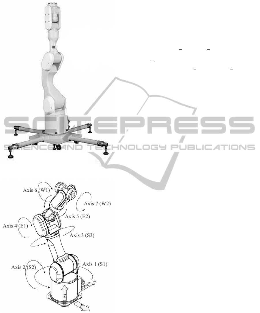
Figure 2: Mitsubishi PA10-7CE robot arm.
Figure 3: Mitsubishi PA10-7CE robot axes.
u(k) =
h
u
1
u
2
u
3
u
4
u
5
u
6
u
7
i
⊤
x
1
d
(k) =
h
x
1
1
d
x
1
2
d
x
1
3
d
x
1
4
d
x
1
5
d
x
1
6
d
x
1
7
d
i
⊤
χ
1
i
(k) = x
1
i
(k)
(21)
where x
1
1
d
(k) to x
1
7
d
(k) are the desired trajectory sig-
nals. The control objective is to drive the output χ
1
i
(k)
to track the reference x
1
i
d
(k). Using (21), the system
(20) can be represented in the block strict feedback
form as
x
1
i
(k+ 1) = f
1
i
(x
1
i
(k)) + g
1
i
(x
1
i
(k))x
2
i
(k)
x
2
i
(k+ 1) = f
2
i
(x
2
i
(k)) + g
2
i
(x
2
i
(k))u
i
(k)
(22)
where x
2
i
(k) =
x
1
i
(k) x
2
i
(k)
⊤
, i = 1,... ,7,
f
1
i
(x
1
i
(k)), g
1
i
(x
1
i
(k)), f
2
i
(x
2
i
(k)) and g
2
i
(x
2
i
(k)) are
assumed to be unknown. To this end, we use a
HONN to approximate the desired virtual controls
and the ideal practical control described as
α
1∗
i
(k) , x
2
i
(k) = ϕ
1
i
(x
1
i
(k),x
1
i
d
(k+ 2))
u
∗
i
(k) = ϕ
1
i
(x
1
i
(k),x
2
i
(k),α
1∗
i
(k))
χ
1
i
(k) = x
1
i
(k).
(23)
The HONN proposed for this application is as fol-
lows:
α
1∗
i
(k) = w
1⊤
i
S
1
i
(z
1
i
(k))
u
i
(k) = w
2⊤
i
S
2
i
(z
2
i
(k))
(24)
with
z
1
i
(k) = [x
1
i
(k),x
1
i
d
(k+ 2)]
z
2
i
(k) = [x
1
i
(k),x
2
i
(k),α
1
i
(k)].
(25)
The weights are updated using the EKF (13) - (19)
with i = 1, 2 and
e
1
i
(k) = x
1
i
d
(k) − χ
1
i
(k)
e
2
i
(k) = x
2
i
(k) − α
1
i
(k).
(26)
The training is performed on-line using a series-
parallel configuration. All the neural network states
are initialized in a random way.
6 SIMULATION RESULTS
For simulation, we select the following discrete-time
trajectories (Ramirez, 2008)
x
1
1
d
(k) = c
1
(1− e
d
1
kT
3
)sin(ω
1
kT)[rad]
x
1
2
d
(k) = c
2
(1− e
d
2
kT
3
)sin(ω
2
kT)[rad]
x
1
3
d
(k) = c
3
(1− e
d
3
kT
3
)sin(ω
3
kT)[rad]
x
1
4
d
(k) = c
4
(1− e
d
4
kT
3
)sin(ω
4
kT)[rad]
x
1
5
d
(k) = c
5
(1− e
d
5
kT
3
)sin(ω
5
kT)[rad]
x
1
6
d
(k) = c
6
(1− e
d
6
kT
3
)sin(ω
6
kT)[rad]
x
1
7
d
(k) = c
7
(1− e
d
7
kT
3
)sin(ω
7
kT)[rad]
(27)
NCTA 2011 - International Conference on Neural Computation Theory and Applications
86
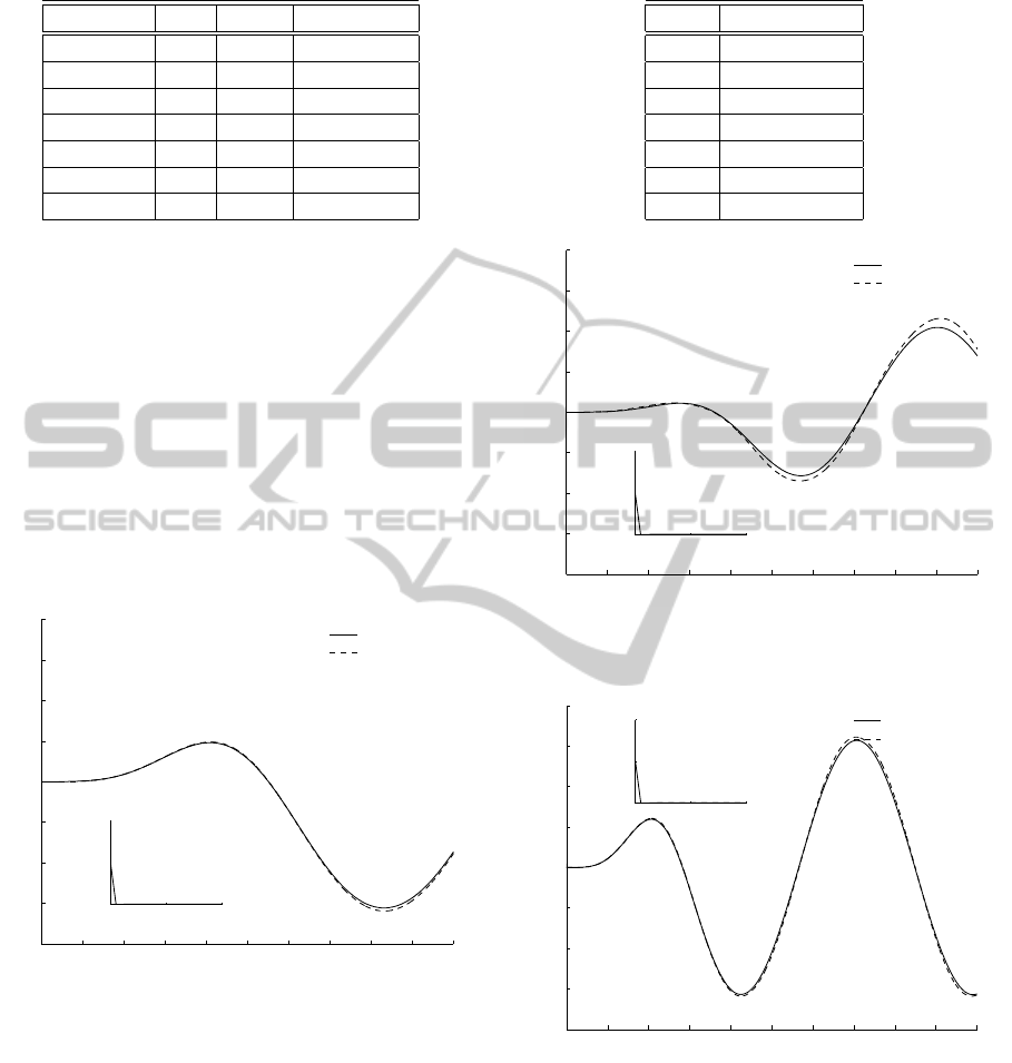
Table 1: Parameters for desired trajectories.
i-th Joint c
i
d
i
ω
i
1 π/2 0.001 0.285 rad/s
2 π/3 0.001 0.435 rad/s
3 π/2 0.01 0.555 rad/s
4 π/3 0.01 0.645 rad/s
5 π/2 0.01 0.345 rad/s
6 π/3 0.01 0.615 rad/s
7 π/2 0.01 0.465 rad/s
the selected parameters c, d and ω for desired trajecto-
ries of each joint are shown in Table 1. The sampling
time is selected as T = 1 millisecond.
These selected trajectories (27) incorporate a si-
nusoidal term to evaluate the performance in presence
of relatively fast periodic signals, for which the non-
linearities of the robot dynamics are really important.
Simulation results for trajectory tracking using the
decentralized neural backstepping control (DNBS)
scheme are shown in Figs. 4 to Fig. 10. The ini-
tial conditions for the plant are different that those of
the desired trajectory. According to these figures, the
tracking errors for all joints present a good behavior
and remain bounded as shown in Fig. 11.
0 2 4 6 8 10 12 14 16 18 20
−2
−1.5
−1
−0.5
0
0.5
1
1.5
2
Time (s)
Position (rad)
↑ Initial condition
x
1
1d
Desired trajectory
χ
1
1
Plant
0 0.01 0.02
0
0.05
0.1
← x
1
1d
(0)=0.05
Time(s)
Position (rad)
Figure 4: Trajectory tracking for joint 1 x
1
1
d
(k) (solid line)
and χ
1
1
(k) (dashed line).
The applied torques to each joint are always inside
of the prescribed limits given by the actuators manu-
facturer (see Table 2); that is, their absolute values are
smaller than the bounds τ
max
1
to τ
max
7
, respectively.
7 CONCLUSIONS
In this paper a decentralized neural control scheme
based on the backstepping technique is presented.
The control law for each joint is approximated by a
Table 2: Maximum torques.
Joint Max Torque
1 232 N-m
2 232 N-m
3 100 N-m
4 100 N-m
5 14.5 N-m
6 14.5 N-m
7 14.5 N-m
0 2 4 6 8 10 12 14 16 18 20
−2
−1.5
−1
−0.5
0
0.5
1
1.5
2
Time (s)
Position (rad)
↑ Initial condition
x
1
2d
Desired trajectory
χ
1
2
Plant
0 0.01 0.02
0
0.05
0.1
← x
1
2d
(0)=0.05
Time(s)
Position (rad)
Figure 5: Trajectory tracking for joint 2 x
1
2
d
(k) (solid line)
and χ
1
2
(k) (dashed line).
0 2 4 6 8 10 12 14 16 18 20
−2
−1.5
−1
−0.5
0
0.5
1
1.5
2
Time (s)
Position (rad)
↑ Initial condition
x
1
3d
Desired trajectory
χ
1
3
Plant
0 0.01 0.02
0
0.05
0.1
← x
1
3d
(0)=0.05
Time(s)
Position (rad)
Figure 6: Trajectory tracking for joint 3 x
1
3
d
(k) (solid line)
and χ
1
3
(k) (dashed line).
high order neural network. The training of each neu-
ral network is performed on-line using an extended
Kalman filter. Simulations results for trajectory track-
ing using a seven DOF PA10-7CE Mitsubishi robot
arm show the effectiveness of the proposed control
scheme.
DECENTRALIZED NEURAL BACKSTEPPING CONTROL FOR AN INDUSTRIAL PA10-7CE ROBOT ARM
87
0 2 4 6 8 10 12 14 16 18 20
−2
−1.5
−1
−0.5
0
0.5
1
1.5
2
Time (s)
Position (rad)
↑ Initial condition
x
1
4d
Desired trajectory
χ
1
4
Plant
0 0.01 0.02
0
0.05
0.1
← x
1
4d
(0)=0.05
Time(s)
Position (rad)
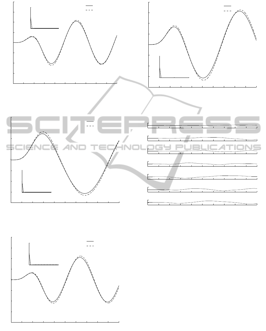
Figure 7: Trajectory tracking for joint 4 x
1
4
d
(k) (solid line)
and χ
1
4
(k) (dashed line).
0 2 4 6 8 10 12 14 16 18 20
−2
−1.5
−1
−0.5
0
0.5
1
1.5
2
Time (s)
Position (rad)
↑ Initial condition
x
1
5d
Desired trajectory
χ
1
5
Plant
0 0.01 0.02
0
0.05
0.1
← x
1
5d
(0)=0.05
Time(s)
Position (rad)
Figure 8: Trajectory tracking for joint 5 x
1
5
d
(k) (solid line)
and χ
1
5
(k) (dashed line).
0 2 4 6 8 10 12 14 16 18 20
−2
−1.5
−1
−0.5
0
0.5
1
1.5
2
Time (s)
Position (rad)
↑ Initial condition
x
1
6d
Desired trajectory
χ
1
6
Plant
0 0.01 0.02
0
0.05
0.1
← x
1
6d
(0)=0.05
Time(s)
Position (rad)
Figure 9: Trajectory tracking for joint 6 x
1
6
d
(k) (solid line)
and χ
1
6
(k) (dashed line).
0 2 4 6 8 10 12 14 16 18 20
−2
−1.5
−1
−0.5
0
0.5
1
1.5
2
Time (s)
Position (rad)
↑ Initial condition
x
1
7d
Desired trajectory
χ
1
7
Plant
0 0.01 0.02
0
0.05
0.1
← x
1
7d
(0)=0.05
Time(s)
Position (rad)
Figure 10: Trajectory tracking for joint 7 x
1
7
d
(k) (solid line)
and χ
1
7
(k) (dashed line).
0 2 4 6 8 10 12 14 16 18 20
−0.2
0
0.2
Time (s)
Error (rad)
e
1
1Track
0 2 4 6 8 10 12 14 16 18 20
−0.2
0
0.2
Time (s)
Error (rad)
e
1
2Track
0 2 4 6 8 10 12 14 16 18 20
−0.2
0
0.2
Time (s)
Error (rad)
e
1
3Track
0 2 4 6 8 10 12 14 16 18 20
−0.2
0
0.2
Time (s)
Error (rad)
e
1
4Track
0 2 4 6 8 10 12 14 16 18 20
−0.2
0
0.2
Time (s)
Error (rad)
e
1
5Track
0 2 4 6 8 10 12 14 16 18 20
−0.2
0
0.2
Time (s)
Error (rad)
e
1
6Track
0 2 4 6 8 10 12 14 16 18 20
−0.2
0
0.2
Time (s)
Error (rad)
e
1
7Track
Figure 11: Tracking errors for joints 1 to 7.
ACKNOWLEDGEMENTS
The first author thanks to Universidad Autonoma
del Carmen (UNACAR) and the Programa de Mejo-
ramiento del Profesorado (PROMEP-MEXICO) for
supporting this research.
REFERENCES
Alanis, A. Y., Sanchez, E. N., and Loukianov, A. G. (2007).
Discrete-time adaptive backstepping nonlinear control
via high-order neural networks. IEEE Transactions on
Neural Networks, 18(4):1185–1195.
Ge, S. S., Zhang, J., and Lee, T. H. (2004). Adaptive
neural network control for a class of MIMO nonlin-
ear systems with disturbances in discrete-time. IEEE
Transactions on Systems, Man, and Cybernetics Part
B, 34(4):1630–1645.
Higuchi, M., Kawamura, T., Kaikogi, T., Murata, T., and
NCTA 2011 - International Conference on Neural Computation Theory and Applications
88

Kawaguchi, M. (2003). Mitsubihi clean room robot.
Tecnical review, Mitsubishi Heavy Industries, Ltd.
Huang, S., Tan, K. K., and Lee, T. H. (2003). Decentralized
control design for large-scale systems with strong in-
terconnections using neural networks. IEEE Transac-
tions on Automatic Control, 48(5):805–810.
Jamisola, R. S., Maciejewski, A. A., and Roberts, R. G.
(2004). Failure-tolerant path planning for the PA-10
robot operating amongst obstacles. In Proceedings of
IEEE International Conference on Robotics and Au-
tomation, pages 4995–5000, New Orleans, LA, USA.
Karakasoglu, A., Sudharsanan, S. I., and Sundareshan,
M. K. (1993). Identification and decentralized adap-
tive control using dynamical neural networks with ap-
plication to robotic manipulators. IEEE Transactions
on Neural Networks, 4(6):919–930.
Kennedy, C. W. and Desai, J. P. (2003). Force feedback us-
ing vision. In Proceedings of IEEE International Con-
ference on Advanced Robotics, Co´ımbra, Portugal.
Krstic, M., Kanellakopoulos, I., and Kokotovic, P. (1995).
Nonlinear and Adaptive Control Design. John Wiley
& Sons, Inc, New York, USA.
Liu, M. (1999). Decentralized control of robot manipula-
tors: nonlinear and adaptive approaches. IEEE Trans-
actions on Automatic Control, 44(2):357–363.
Ni, M. L. and Er, M. J. (2000). Decentralized control of
robot manipulators with coupling and uncertainties.
In Proceedings of the American Control Conference,
pages 3326–3330, Chicago, Illinois, USA.
Ramirez, C. (2008). Dynamic modeling and torque-mode
control of the Mitsubishi PA10-7CE robot. Master
dissertation (in spanish), Instituto Tecnol´ogico de la
Laguna, Torre´on, Coahuila, Mexico.
Rovithakis, G. A. and Christodoulou, M. A. (2000). Adap-
tive Control with Recurrent High-Order Neural Net-
works. Springer, London, U.K.
Safaric, R. and Rodic, J. (2000). Decentralized neural-
network sliding-mode robot controller. In Proceed-
ings of 26th Annual Conference on the IEEE Indus-
trial Electronics Society, pages 906–911, Nagoya,
Aichi, Japan.
Sanchez, E. N. and Ricalde, L. J. (2003). Trajectory track-
ing via adaptive recurrent neural control with input
saturation. In Proceedings of International Joint Con-
ference on Neural Networks, pages 359–364, Port-
land, Oregon, USA.
Santiba˜nez, V., Kelly, R., and Llama, M. A. (2005). A
novel global asymptotic stable set-point fuzzy con-
troller with bounded torques for robot manipulators.
IEEE Transactions on Fuzzy Systems, 13(3):362–372.
Song, Y. and Grizzle, J. W. (1995). The extended Kalman
filter as local asymptotic observer for discrete-time
nonlinear systems. Journal of Mathematical Systems,
Estimation and Control, 5(1):59–78.
DECENTRALIZED NEURAL BACKSTEPPING CONTROL FOR AN INDUSTRIAL PA10-7CE ROBOT ARM
89
