
USING THE GNG-M ALGORITHM TO DEAL WITH THE
PROBLEM OF CATASTROPHIC FORGETTING IN
INCREMENTAL MODELLING
H´ector F. Satiz´abal M. and Andres Perez-Uribe
University of Applied Sciences of Western Switzerland (HEIG-VD), Del´emont, Switzerland
Keywords:
Catastrophic Interference, Incremental task, Incremental learning, Sequential learning, Growing neural gas.
Abstract:
Creating computational models from large and growing datasets is an important issue in current machine
learning research, because most modelling approaches can require prohibitive computational resources. This
work presents the use of incremental learning algorithms within the framework of an incremental modelling
approach. In particular, it presents the GNG-m algorithm, an adaptation of the Growing Neural Gas algorithm
(GNG), capable of circumventing the problem of catastrophic forgetting when modelling large datasets in a
sequential manner. We illustrate this by comparing the performance of GNG-m with that of the original GNG
algorithm, on a vector quantization task. Last but not least, we present the use of GNG-m in an incremental
modelling task using a real-world database of temperature, coming from a geographic information system
(GIS). The dataset of more than one million multidimensional observations is split in seven parts and then
reduced by vector quantization to a codebook of only thousands of prototypes.
1 INTRODUCTION
Building computationalmodels by means of inductive
inference has always been an important issue in sci-
ence. Current information systems gather information
in databases containing huge amounts of data, mak-
ing difficult to tackle the problem of modelling by us-
ing traditional methods. Additionally, one must care
about the fact that, most of the time, these databases
continuously grow, thus requiring a dynamic mod-
elling approach being able to add new knowledge to
pre-existent models. As an example, consider mod-
elling a biological process, e.g., growth or develop-
ment. Biological processes change over time due to
the continuous variations on stimuli (e.g., climate).
Plants and animals behavedifferentdependingon sea-
sons, and seasons evolve through years depending on
more complex processes (e.g., global warming). This
is the intrinsic complexity of the problem, but this
scenario is reinforced by the fact that it is not pos-
sible to have all the concerned data in advance. In-
stead, the data are gradually collected in an incre-
mental way generating growing databases. Creating a
model of a such process each time new data are gen-
erated could imply large computation time because,
in a static modelling framework, the new model must
be created from scratch using the whole set of data.
A dynamic approach with growing models incorpo-
rating the information of new data is desirable in this
case.
An interesting approach which deals with this
kind of datasets is incremental modelling. This mod-
elling paradigm consists in considering the modelling
problem as an incremental task (Giraud-Carrier,
2000), and then using incremental learning tech-
niques in order to build a model from the available
data. Therefore, by using this approach, huge datasets
may be processed when they are still growing or, they
might be transformed by means of a sampling or par-
titioning procedure
1
before being fed to the incremen-
tal modelling framework.
This article presents the use of GNG-m, an adap-
tation of the popular GNG algorithm (Fritzke, 1995),
as a means for achieving incremental learning. More
specifically, the idea of the contribution is to use an
incremental modelling approach in order to process
huge datasets which would require too much mem-
ory and computation resources when using standard
batch approaches. The remainder of the article con-
tains the following sections. Section 2 introduces the
concept of incremental learning, gives some defini-
1
By sampling or splitting the dataset the modelling task
is transformed in an incremental task.
267
F. Satizábal M. H. and Perez-Uriibe A..
USING THE GNG-M ALGORITHM TO DEAL WITH THE PROBLEM OF CATASTROPHIC FORGETTING IN INCREMENTAL MODELLING.
DOI: 10.5220/0003683702670276
In Proceedings of the International Conference on Neural Computation Theory and Applications (NCTA-2011), pages 267-276
ISBN: 978-989-8425-84-3
Copyright
c
2011 SCITEPRESS (Science and Technology Publications, Lda.)

tions, and shows generalities of the approach. Section
3 explains the standard GNG algorithm, as well as the
modifications that were introduced in order to make
it more suitable for incremental modelling. Section 4
shows some tests of the performance of the algorithm
on a toy-set problem, and Section 5 presents the ap-
plication of the algorithm to a real-world large multi-
dimensional dataset. Finally, Section 6 draws some
conclusions about the approach of incremental mod-
elling in the task of processing huge databases, and on
the use of incremental learning algorithms like GNG
in this purpose.
2 INCREMENTAL MODELLING
The fact of having large or growingdatasets, while be-
ing positive and also desirable from the point of view
of a data acquisition system, constitutes a major draw-
back if the data are to be used in inductive modelling.
In the case of a huge database, one can devise two
possibilities. On the one hand, using huge amounts
of data to build models could be prohibitive because
of computational or storage constraints. And on the
other hand, taking only partial information from the
complete set and use it to build a model, implies the
use of special modelling paradigms being able to ap-
pend or insert new information into partial or growing
adaptive models.
A similar landscape is depicted if one thinks on
growing databases. It is a matter of fact that in order
to build an accurate model, a large enough amount of
data must be available. There are also two difficulties
here. On the one hand, it is not a trivial issue to know
beforehand the amount of data that is large enough for
building a model, and this is even more difficult if the
data collecting process is still running. On the other
hand, suppose that the amount of gathered informa-
tion is large enough to build a model. In the case of
having a static process as modelling objective, those
data would be sufficient to reach some level of accu-
racy. Conversely, if the model should fit a dynamic
process, it would be better to have an adaptive mod-
elling framework that follows the changes of the pro-
cess, instead of having absolute stable models which
have to be rebuilt from scratch each time the process
changes. Again, a model structure that incrementally
changes with the amount and quality of data might be
a good strategy.
A modelling framework which fulfils the afore-
said requirements is incremental modelling, also
called incremental learning. In the area of ma-
chine learning, the term incremental learning has syn-
onymously been used with pattern learning and on-
line learning to describe the opposite of batch learn-
ing (Chalup, 2002). Within this context, it only means
to distinguish two policies for modifying the param-
eters of a model during training i.e., after the presen-
tation of each training example in the online case, or
after the cumulation of a certain number of modifica-
tions in the batch case. We are considering a more
specific definition of the concept of incremental mod-
elling, which will be explained after defining the con-
cept of incremental task in the next subsection.
2.1 Incremental Task
In general, modelling tasks where the examples or ob-
servations become available over time (usually one
at a time) are considered as incremental learning
tasks (Giraud-Carrier, 2000).
Traditional static methods can be employed for
building a model from an incremental task given that,
if there exist the possibility of waiting for the data,
any incremental learning task can be transformed into
a non-incremental one (Giraud-Carrier, 2000). This
approach has the hindrance of reaching excessive vol-
umes of data that could render infeasible the mod-
elling task. It would be preferable to make use of
the advantages of incremental learners in this case. In
the same way, a large non-incremental modelling task
being unbearable by traditional modelling approaches
can be transformed into an incremental task by sam-
pling or splitting the data, and then to use a incremen-
tal learner in order to build a model from the obtained
incremental dataset.
2.2 Incremental Learning
Besides being a synonym of pattern learning or on-
line learning in the machine learning terminology, in-
cremental learning is a concept which has been as-
sociated with learning processes where a standard
learning mechanism is combined with or is influenced
by stepwise adjustments during the learning process.
These adaptations can be changes in the structure
of the learning system (e.g., growing and construc-
tive neural networks), or changes in its parameters
(e.g., stochastic learning), or even changes in the con-
stitution of its input signals (e.g., order, complex-
ity) (Chalup, 2002). These adaptations have the pur-
pose of enabling the construction of more specialized
models by adding new information to the already ex-
istent knowledge, when it is available.
Within this context, incremental learning shares
the same meaning of sequential learning. In se-
quential learning, the learning system is sequentially
trained by using different datasets, which most of the
NCTA 2011 - International Conference on Neural Computation Theory and Applications
268
times are chunks of a larger dataset that grows due to
a gathering process which is still running. This defini-
tion is very close to the concept of online learning, ex-
cept but the fact that in pure sequential learning each
dataset (and all related information) is discarded after
each step of the sequence. Only the model parameters
are kept
2
(Sarle, 2002).
Thus, as a conclusion, incremental modelling may
be defined as the process of using any incremental
or sequential learning algorithm, to solve any incre-
mental learning task, even those which comes from
the transformation of non-incrementalones. This arti-
cle emphasizes on the use of incremental learning for
solving non-incremental tasks that were transformed
into incremental ones by means of a sampling or par-
tition procedure.
2.2.1 Stability - Plasticity Dilemma
Incremental learning algorithms must be designed to
remain plastic in response to significant new events,
yet also remain stable in response to irrelevant events.
Moreover, it is desirable that, in the plastic mode
of the model, the new events affect only the part of
the model being concerned with the new knowledge
without causing interference with pre-existent con-
cepts. This compromise between stability and plastic-
ity (Grossberg, 1987; Carpenter and Grossberg, 1987)
is difficult to achieve in static models with distributed
representations which try to minimize an objective
function. This phenomenonis due to the fact that sub-
sequent training datasets may have totally different
local minima, making the sequential training of suc-
cessive datasets to forget all previous sets, resulting
in the so called catastrophic interference (McCloskey
and Cohen, 1989). Several strategies has been pro-
posed in order to minimize these effects (French,
1994; Robins, 2004) in distributed representations.
Besides a distributed representation, information
can also be represented using a local scheme. Lo-
cal encoding of the information is one of the require-
ments to successfully perform learning in a sequential
manner (Sarle, 2002). The use of models with a local
representation of the information allows partial up-
dates of their parameters, permitting new knowledge
to be introduced into the model without modifying the
previous information already stored. Moreover, lo-
cal adaptations must be accompanied by the ability of
dynamically changing the model structure (i.e., grow-
ing), in order to give enough flexibility when required.
2
In the particular case of artificial neural networks, these
parameters are the weighted connections between neurons
if knowledge is encoded in a distributed manner, or unit po-
sitions if the encoding schema is local.
3 THE GROWING NEURAL GAS
ALGORITHM
Growing Neural Gas (GNG) (Fritzke, 1995) is an
incremental point-based network (Bouchachia et al.,
2007) that performs vector quantization and topology
learning. The algorithm builds a neural network by in-
crementally adding units using a competitiveHebbian
learning strategy. The resulting structure is a graph of
neurons that reproduces the topology of the dataset by
keeping the distribution and the dimensionality of the
training data (Fritzke, 1997).
The classification performance of GNG is com-
parable to conventional approaches (Heinke and
Hamker, 1998) but has the advantage of being incre-
mental. Hence, giving the possibility of training the
network even if the dataset is not completely available
all the time while reducing the risk of catastrophic in-
terference by using local encoding.
The algorithm proposed by Fritzke is shown in Ta-
ble 1. In this algorithm, every λ iterations (step 8)
one unit is inserted halfway between the unit q having
the highest error and its neighbour f having also the
highest error. Carrying out this insertion makes the
network to converge to a structure where each cell is
the prototype for approximately the same number of
data points and hence, keeping the original data dis-
tribution. The term “nearest unit” in step 2 refers to
the more widely used concept of best matching unit
(BMU).
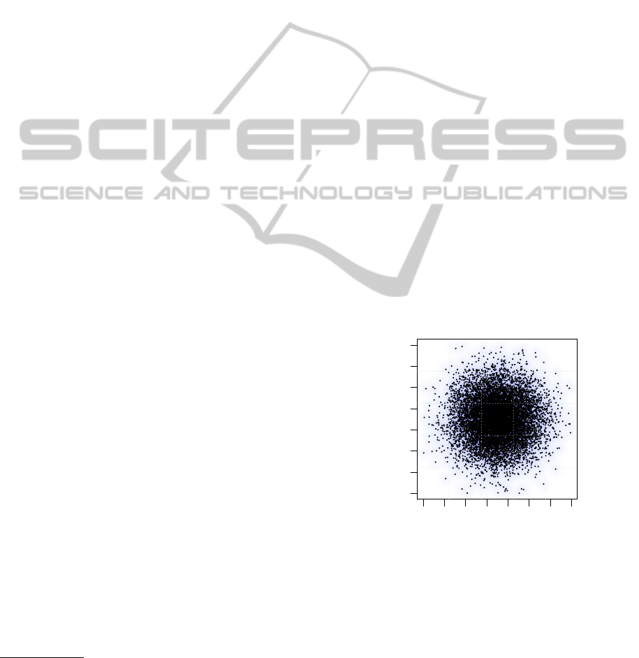
−2 0 2 4 6 8 10
−2 0 2 4 6 8 10
X
Y
Figure 1: Two-dimensional Single-blob normal distribu-
tion.
As an example, a GNG network was trained using
the dataset shown in Figure 1, and the training param-
eters shown in Table 2. These values were selected af-
ter several runs of the algorithm. This dataset contains
10’000 observations drawn from a two-dimensional
normal distribution with means µ
x
= 5, µ
y
= 5 and
standard deviations σ
x
= 2, σ
y
= 2.
Figure 2 shows the position and distribution of
USING THE GNG-M ALGORITHM TO DEAL WITH THE PROBLEM OF CATASTROPHIC FORGETTING IN
INCREMENTAL MODELLING
269
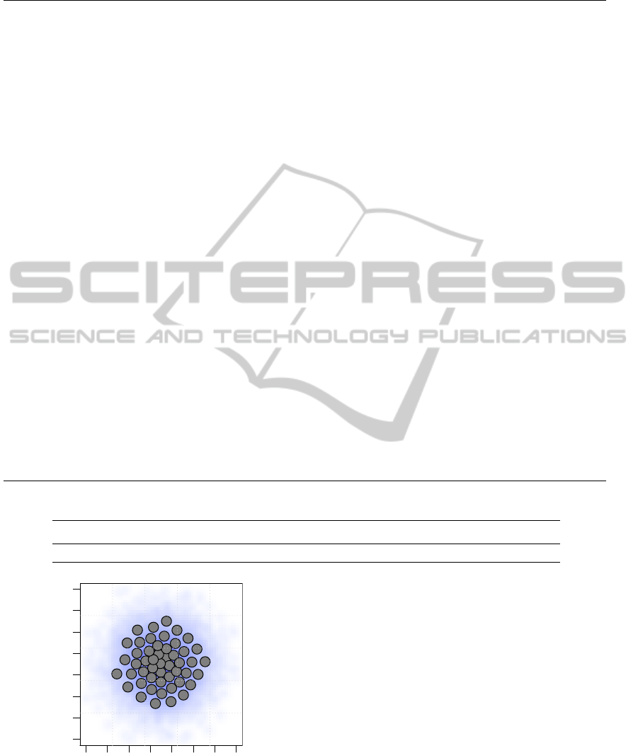
Table 1: Original growing neural gas algorithm proposed by Fritzke.
Step 0: Start with two units a and b at random positions w
a
and w
b
in ℜ
n
Step 1: Generate an input signal ξ according to a (unknown) probability density function
P(ξ)
Step 2: Find the nearest unit s
1
and the second-nearest unit s
2
Step 3: Increment the age of all edges emanating from s
1
Step 4: Add the squared distance between the input signal and the nearest unit in input space
to a local counter variable:
∆error(s
1
) = kw
s
1
− ξk
2
Step 5: Move s
1
and its direct topological neighbours towards the input signal ξ by fractions
ε
b
and ε
n
, respectively, of the total distance:
∆w
s
1
= ε
b
(ξ− w
s
1
)
∆w
n
= ε
n
(ξ− w
n
) for all direct neighbours n of s
1
Step 6: If s
1
and s
2
are connected by an edge, set the age of this edge to zero. If such an
edge does not exist, create it
Step 7: Remove edges with an age larger than a
max
. If the remaining units have no emanat-
ing edges, remove them as well
Step 8: If the number of input signals generated so far is an integer multiple of a parameter
λ, insert a new unit as follows:
• Determine the unit q with the maximum accumulated error.
• Insert a new unit r halfway between q and its neighbour f with the largest error
variable: w
r
= 0.5
w
q
+ w
f
• Insert edges connecting the new unit r with units q and f, and remove the
original edge between q and f.
• Decrease the error variables of q and f by multiplying them with a constant α.
Initialize the error variable of r with the new value of the error variable of q.
Step 9: Decrease all error variables by multiplying them with a constant d
Step 10: If a stopping criterion (e.g., net size or some performance measure) is not yet ful-
filled go to step 1
Table 2: Parameters for the Growing Neural Gas algorithm.
Parameter ε
b
ε
n
λ a
max
α d
value 0.005 0.001 500 100 0.5 0.9
−2 0 2 4 6 8 10
−2 0 2 4 6 8 10
X
Y
Figure 2: Prototype vectors obtained with the GNG algo-
rithm using the whole dataset.
the 50 cells of the resulting structure. A smoothed
coloured density representation of the dataset from
where the prototypes were obtained was added to ev-
ery scatter plot in this paper. Showing the original
distribution of the training data can be useful to eval-
uate if the prototypes were correctly placed after the
learning process. As we can see in Figure 2, the dis-
tribution of each one of the variables is reproduced by
the group of prototypes in the network.
Now, in order to simulate the conditions that
would require the use of incremental modelling, let
us consider this dataset to be so huge that it is impos-
sible to be processed in one single step due to memory
constraints. Then, incremental modelling arises as a
possible solution to overcome this problem. The huge
dataset can be split, transforming the task of mod-
elling into an incremental one, and then one can use
an incremental learner (e.g., the GNG algorithm) to
build a model of the dataset in a sequential manner.
Figure 3 shows the resulting positions of the pro-
NCTA 2011 - International Conference on Neural Computation Theory and Applications
270
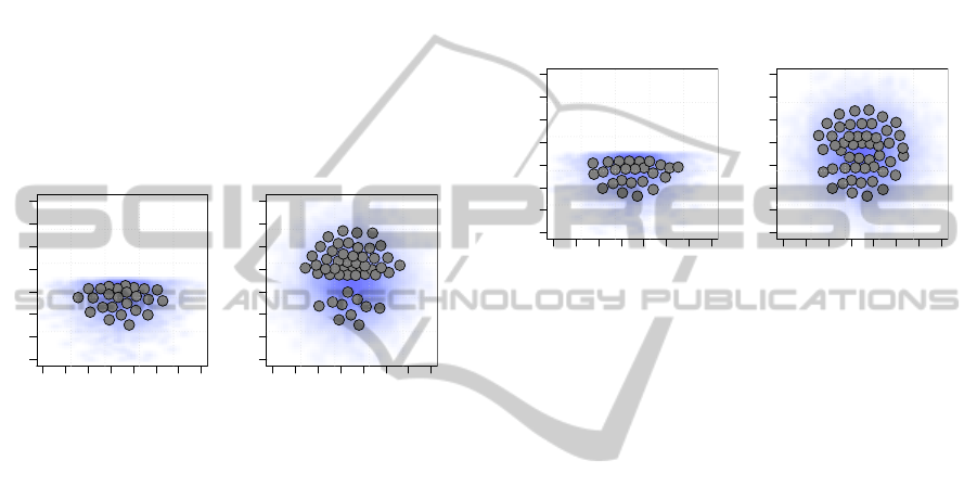
totypes of the GNG network after doing a sequential
training with the split version (2 parts) of the dataset
shown in Figure 1. As it can be seen, after the first
step of the sequence, the algorithm reproducesthe dis-
tribution of the first part of the dataset without any
problem. Then, after presenting the second part, the
algorithm “forgets” the first part (i.e., the quantization
error for this part increases), assigning some of the
prototypes that represented the first part of the data to
the more recent second part of the dataset. This unde-
sirable manifestation of catastrophic forgetting is due
to the fact that the algorithm, being pure incremen-
tal, does not keep information about previous datasets
used to train the network, and therefore, there is no
way of knowing if one of the units of the network rep-
resented some important data, and that given this fact
its position must remain invariable.
−2 0 2 4 6 8 10
−2 0 2 4 6 8 10
X
Y
(a) Step 1
−2 0 2 4 6 8 10
−2 0 2 4 6 8 10
X
Y
(b) Step 2
Figure 3: Prototypes generated with the sequential training
of a GNG from a dataset split in two parts.
In order to minimize the aforementioned situation,
one modification to the original algorithm is proposed
in Section 3.1.
3.1 The GNG-m Algorithm
The original version of the GNG algorithm does not
keep any additional information about the observa-
tions that have been presented to the network; only
unit positions and edge ages are stored in the model.
This policy, while making the algorithm suitable for
performing incremental learning (pure sequential al-
gorithm), does not allow the algorithm to know if a
unit in the graph has been an important prototype (i.e.,
a best matching unit) in previous runs.
The idea of the GNG-m algorithm is to attenuate
parameters ε
b
and ε
n
of the original version (which
represent the change of position of the units) for the
units which have been useful for representing obser-
vations previously presented to the network. In order
to do that, we associated a property of “mass” to each
unit in the network, in a way that units having been
useful for quantizing the dataset get more mass than
units representing less data. Hence, we adapted step 5
to take into account the mass value of the unit, freeing
“lighter” units and locking the “heavier” ones.
In summary, the proposed modification adds two
parameters, massInc, and massDec, to the original
GNG algorithm. Each time a unit is selected as the
nearest unit s
1
, its mass is incremented by massInc,
while all its direct neighbours decrease their mass by
massDec. The mass of the unit is then used to mod-
ulate how far a unit can move in a single step, and as
a result, units having been selected more often as the
nearest unit change less their position than units that
represent less points in the dataset.
−2 0 2 4 6 8 10
−2 0 2 4 6 8 10
X
Y
(a) Step 1
−2 0 2 4 6 8 10
−2 0 2 4 6 8 10
X
Y
(b) Step 2
Figure 4: Prototypes generated with the sequential training
of a GNG-m from a dataset split in two parts.
As an example, Figure 4 shows the resulting po-
sitions of the prototypes of the GNG-m network after
doing a sequential training with the split version (2
parts) of the dataset shown in Figure 1. Contrary to
the results shown in Section 3, the modified version
of the algorithm satisfactorily places new prototypes
when the second part of the file is presented, with-
out modifying the positions of the prototypes repre-
senting the first part. More examples using this new
algorithm are given in the next section.
4 TOY-SET EXPERIMENTS
This section shows the results of several tests using
the dataset shown in Figure 1. Two approaches for
modelling a huge dataset are compared i.e., model
merging and incremental modelling. In the case of
model merging, we explored parallel and cascade
merging. For the incremental modelling approach, we
used both versions of the GNG algorithm presented in
Section 3 and Section 3.1.
In the case of this toy-set, it is possible to train a
model with the whole database. Thus, in order to have
a reference to compare with, the resulting prototypes
when using the whole dataset are shown in Figure 2.
The dataset used for the tests has only 10’000 ob-
servations; however, we used it in order to simulate a
huge one which cannot be loaded in memory. In order
USING THE GNG-M ALGORITHM TO DEAL WITH THE PROBLEM OF CATASTROPHIC FORGETTING IN
INCREMENTAL MODELLING
271
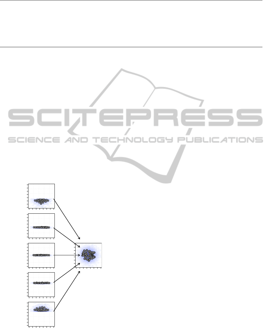
Table 3: Proposed modification to the original algorithm.
Step 5: Move s
1
and its direct topological neighbours towards the input signal ξ by fractions
ε
b
and ε
n
, respectively, of the total distance:
∆w
s
1
= (ε
b
· e
mass
s
1
)(ξ− w
s
1
)
∆w
n
= (ε
n
· e
mass
n
)(ξ− w
n
) for all direct neighbours n of s
1
mass
s
1
= mass
s
1
+ massInc
mass
n
= mass
n
− massDec for all direct neighbours n of s
1
to do that, this toy-set was split in five and four parts
by using different patterns (vertical and tangential re-
spectively).
4.1 Splitting the Dataset in Five Parts
In this first group of experiments the dataset was ver-
tically split in five parts, and each part was used to
build a quantized version of the whole set of observa-
tions in an incremental manner.
4.1.1 Parallel and Cascade Merging
The first approach we explored for accomplishing the
task of building a quantized version of the split dataset
is to train small individual models with each part, and
then to use the resulting prototypes as inputs for train-
ing a final neural network. This final model should
reproduce the distribution of the whole dataset.
−2 2 4 6 8 12
−2 2 4 6 8 12
−2 2 4 6 8 12
−2 2 4 6 8 12
−2 2 4 6 8 12
−2 2 4 6 8 12
−2 2 4 6 8 12
−2 2 4 6 8 12
−2 2 4 6 8 12
−2 2 4 6 8 12
−2 2 4 6 8 12
−2 2 4 6 8 12
X
Y
Figure 5: Prototypes of a GNG after a parallel merging of
five sets of pre-computed prototypes.
Figure 5 shows the results of training five mod-
els (i.e., one model for each one of the parts of the
dataset), and then merging the resulting models into
one single final model. This merging is done by tak-
ing the positions of all the units in the five neural net-
works, and using them as inputs to train a final net-
work with the GNG algorithm. As it can be seen, the
position of the units of the final model reproduces the
input data distribution.
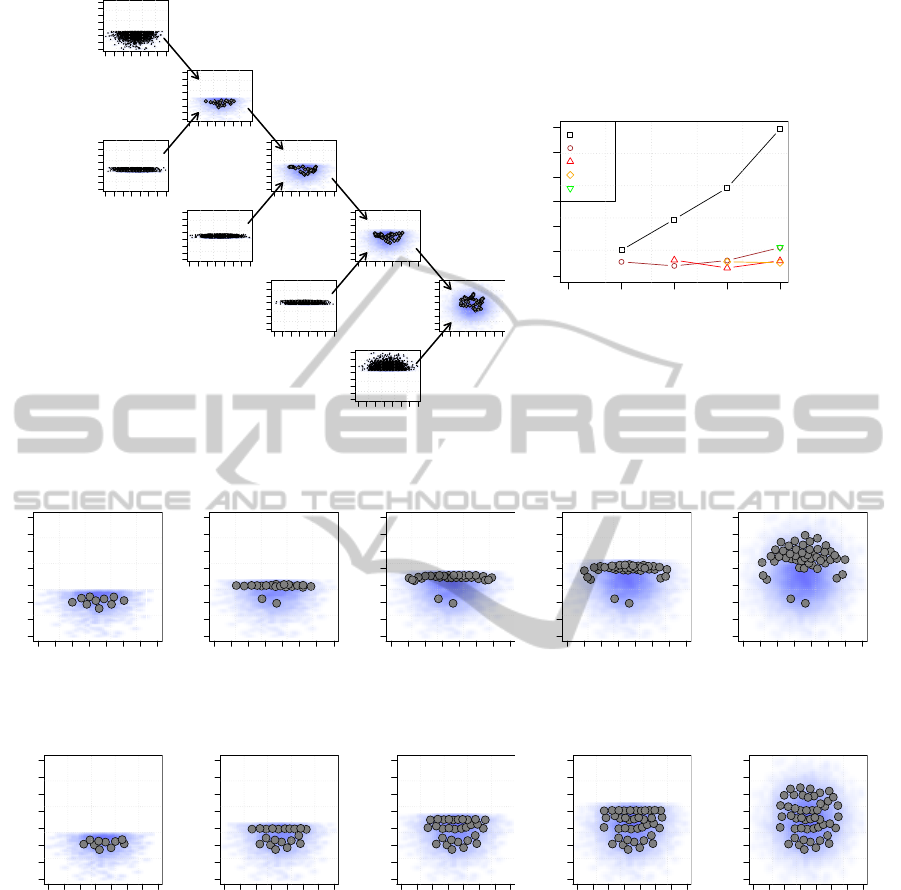
However, this procedure we called parallel merg-
ing, only emulates partially our subject of interest.
The final model can be trained only after having built
each one of the smaller models, or in other words, the
whole dataset must be available in order to have a fi-
nal model reproducing the distribution of the data.
Besides the parallel approach for merging the par-
tial models, we tested a cascade strategy. In this case,
a new up-to-date model is incrementally trained each
time a new part of the dataset is available. There-
fore, a new input dataset must be compiled at each
step of the merging strategy by appending the result-
ing prototypes of the previous step, and the incoming
data. This growing dataset is employed for building
the model at each step.
Figure 6 shows the results of quantizing the pro-
posed dataset by using a cascade merging approach.
As it can be seen in Figure 6(a), the fact of combin-
ing a quantized version of the partial dataset (i.e., the
positions of the units of the last model) with the in-
coming data, does not produce a correct representa-
tion of the whole dataset. The distribution of units in
the GNG algorithm depends strongly on the density of
points in the input dataset. The algorithm distributes
its units in a way that every unit in the network is
a prototype for approximatively the same amount of
data points (i.e., entropy minimization). Hence, the
algorithm gives more importance to the more popu-
lated incoming dataset and tends to “forget” the infor-
mation of the less populated set of prototypes of the
last available model. Figure 6 shows the quantization
error after each step of the cascade merging. As it can
be seen in Figure 6(b), the quantization error of the
first part increases after the presentation of new parts
of the dataset.
NCTA 2011 - International Conference on Neural Computation Theory and Applications
272
−2 2 6 10
−2 2 6 10
X
Y
−2 2 6 10
−2 2 6 10
X
Y
−2 2 6 10
−2 2 6 10
X
Y
Step 2
−2 2 6 10
−2 2 6 10
X
Y
−2 2 6 10
−2 2 6 10
X
Y
Step 3
−2 2 6 10
−2 2 6 10
X
Y
−2 2 6 10
−2 2 6 10
X
Y
Step 4
−2 2 6 10
−2 2 6 10
X
Y
−2 2 6 10
−2 2 6 10
X
Y
Step 5
(a) Cascade merging
1 2 3 4 5
0 1 2 3 4 5 6
Part 1
Part 2
Part 3
Part 4
Part 5
Steps
Average SSE
Quantization error
(b) Quantization error
Figure 6: Prototypes of a GNG after a cascade merging of a dataset split in five parts.
−2 0 2 4 6 8 10
−2 0 2 4 6 8 10
X
Y
(a) Step 1
−2 0 2 4 6 8 10
−2 0 2 4 6 8 10
X
Y
(b) Step 2
−2 0 2 4 6 8 10
−2 0 2 4 6 8 10
X
Y
(c) Step 3
−2 0 2 4 6 8 10
−2 0 2 4 6 8 10
X
Y
(d) Step 4
−2 0 2 4 6 8 10
−2 0 2 4 6 8 10
X
Y
(e) Step 5
Figure 7: Prototypes generated with a sequential training of a GNG from a dataset split in five parts.
−2 0 2 4 6 8 10
−2 0 2 4 6 8 10
X
Y
(a) Step 1
−2 0 2 4 6 8 10
−2 0 2 4 6 8 10
X
Y
(b) Step 2
−2 0 2 4 6 8 10
−2 0 2 4 6 8 10
X
Y
(c) Step 3
−2 0 2 4 6 8 10
−2 0 2 4 6 8 10
X
Y
(d) Step 4
−2 0 2 4 6 8 10
−2 0 2 4 6 8 10
X
Y
(e) Step 5
Figure 8: Prototypes generated with a sequential training of a GNG-m from a dataset split in five parts.
4.1.2 Incremental Modelling with the GNG and
GNG-m Algorithms
In this section we employed the incremental approach
for building a quantized version of the dataset split in
five parts. Figure 7 shows the resulting prototypes
when the dataset is sequentially quantized by using
the original GNG algorithm. As it was already dis-
cussed in section 3, the former parts of the dataset are
lost after presenting the last ones because there is no
information about how useful each unit is in the net-
work.
Figure 9 shows the quantization error for each part
of the dataset after each step of the sequential learning
process. As it can be seen in figure 9(a), the quantiza-
tion error of the former parts increases when the latter
parts of the dataset are presented.
As it was mentioned in Section 3.1, the prob-
lem of catastrophic forgetting can be solved by us-
ing the GNG-m algorithm. Figure 8 shows the result-
ing prototypes after sequentially training a GNG-m
algorithm with the dataset split in five parts. As it
USING THE GNG-M ALGORITHM TO DEAL WITH THE PROBLEM OF CATASTROPHIC FORGETTING IN
INCREMENTAL MODELLING
273
−2 0 2 4 6 8 10
−2 0 2 4 6 8 10
X
Y
(a) Step 1
−2 0 2 4 6 8 10
−2 0 2 4 6 8 10
X
Y
(b) Step 2
−2 0 2 4 6 8 10
−2 0 2 4 6 8 10
X
Y
(c) Step 3
−2 0 2 4 6 8 10
−2 0 2 4 6 8 10
X
Y
(d) Step 4
Figure 10: Prototypes generated with a sequential training of a GNG from a dataset split in four parts.
−2 0 2 4 6 8 10
−2 0 2 4 6 8 10
X
Y
(a) Step 1
−2 0 2 4 6 8 10
−2 0 2 4 6 8 10
X
Y
(b) Step 2
−2 0 2 4 6 8 10
−2 0 2 4 6 8 10
X
Y
(c) Step 3
−2 0 2 4 6 8 10
−2 0 2 4 6 8 10
X
Y
(d) Step 4
Figure 11: Prototypes generated with a sequential training of a GNG from a dataset split in four parts.
1 2 3 4 5
0.0 0.5 1.0 1.5 2.0 2.5
Part 1
Part 2
Part 3
Part 4
Part 5
Steps
Average SSE
Quantization error
(a) Using GNG
1 2 3 4 5
0.0 0.5 1.0 1.5 2.0 2.5
Part 1
Part 2
Part 3
Part 4
Part 5
Steps
Average SSE
Quantization error
(b) Using GNG-m
Figure 9: Average quantization error for each one of the
parts at each step after a sequential training of a dataset split
in five parts.
can be seen, the policy of locking units according to
its relative relevance (mass of the neurons) makes the
algorithm to insert new units where needed, without
modifying units which were useful for representing a
previous subset.
Figure 9 shows the difference between both ver-
sions of the algorithms in terms of the quantization
error of each one of the parts of the dataset. As it can
be seen inFigure 9(b), the quantization error remains
almost constant in the case of the GNG-m algorithm,
whereas the GNG algorithm makes it to continuously
increase.
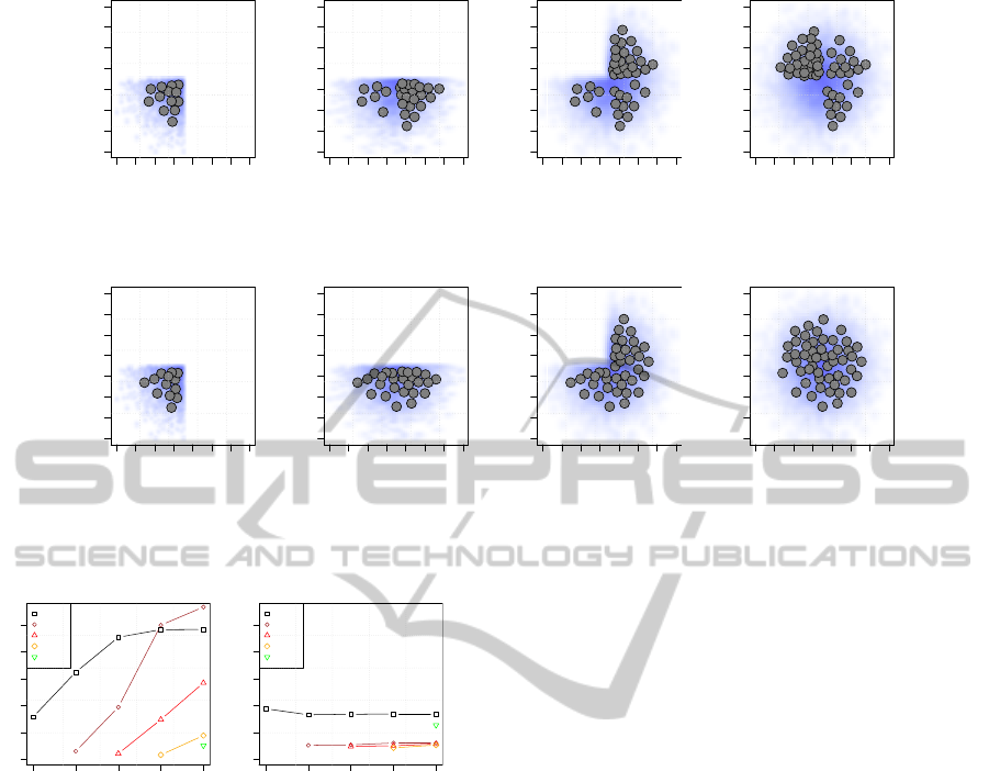
4.2 Splitting the Dataset in Four Parts
This section shows the results of testing the method-
ology by using a version of the dataset which was tan-
gentially split in four parts. This splitting pattern al-
lowed us to test how the algorithm behaves when data
points close to a former distribution are presented in
later stages of the learning sequence. Only results
concerning the incremental modelling approach are
shown in this section.
Figure 10 shows the positions of the resulting pro-
totypes after sequentially applying the original GNG
algorithm to the dataset split in four parts. As it can be
seen, the model loses completely the prototypes rep-
resenting the first part of the dataset after presenting
the last one. Conversely, Figure 11 shows the posi-
tions of the resulting prototypes after using the GNG-
m version of the algorithm. As it can be seen, the
modified version of the algorithm manages to keep
the information of the first part even after presenting
the last part of the dataset. Figure 12 shows the dif-
ference in the behaviour of both versions in terms of
the quantization error of each part of the dataset, after
each step of the sequence.
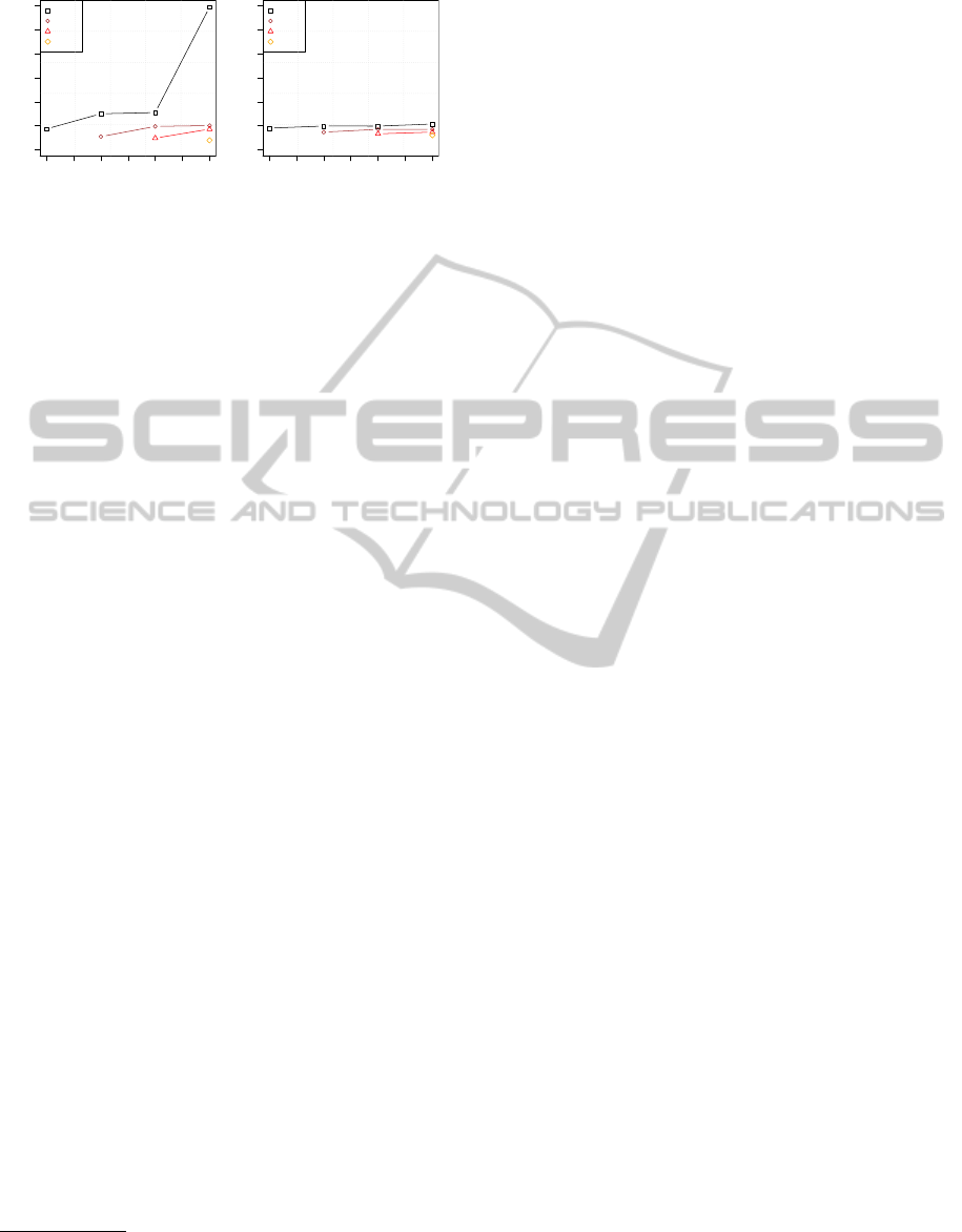
As it can be seen in Figure 12(b), the quantization
error in the GNG-m version of the algorithm remains
almost constant, reducing catastrophic forgetting in
incremental modelling.
5 USING A REAL-WORLD
DATASET
In order to further validate the incremental modelling
approach, and to give an idea of a real application, we
NCTA 2011 - International Conference on Neural Computation Theory and Applications
274
1.0 1.5 2.0 2.5 3.0 3.5 4.0
0.0 0.5 1.0 1.5 2.0 2.5 3.0
Part 1
Part 2
Part 3
Part 4
Steps
Average SSE
Quantization error
(a) Using GNG
1.0 1.5 2.0 2.5 3.0 3.5 4.0
0.0 0.5 1.0 1.5 2.0 2.5 3.0
Part 1
Part 2
Part 3
Part 4
Steps
Average SSE
Quantization error
(b) Using GNG-m
Figure 12: Average quantization error for each one of the
parts at each step after sequential training of the GNG and
GNG-m algorithms with a dataset split in four parts.
quantized a real large multidimensional dataset using
both versions of the GNG algorithm.
The dataset we used comes from the climate
database WORLDCLIM (Hijmans et al., 2005), and
contains information of the current conditions of tem-
perature in Colombia (averaged from 1950 to 2000).
There are 1’336’025 observations, each one corre-
sponding to one pixel with a spatial resolution of one
square kilometre. Each observation has 36 dimen-
sions i.e., maximum temperature for the 12 months of
the year, minimum temperature for the 12 months of
the year, and averagetemperature for the 12 months of
the year. The goal with this dataset is to build a quan-
tized version with a reduced number of prototypes,
which can be analysed faster than taking the whole
set of observations. The resulting set of prototypes
could be useful for finding homologue regions within
the country, or for finding species distributions.
The first step of the process consists in transform-
ing the task of vector quantization into an incremen-
tal task. Thus, the dataset was split in 7 parts
3
, six
parts with 200’000 observations, and one last part
with 136’025 observations. These parts were used
for sequentially training the GNG models. The sec-
ond step in incremental modelling consists in creat-
ing a model from the data by using an incremental
learner algorithm. For this application we did not use
exactly the original version of the GNG algorithm,
but a slightly modified version (Satiz´abal et al., 2009)
which prevents the accumulation of prototypes when
the dataset is highly heterogeneous. The parameters
we used to quantize the data can be found in Table 4.
The resulting prototypes can not be easily visu-
alised given that the dataset has 36 dimensions. In-
stead, in order to illustrate the difference between
both versions of the algorithm, Figure 13 shows the
quantization error of each part of the dataset during
3
The splitting pattern was only geographic, from north
to south, without taking into account the properties of the
dataset in the space of features.
all the steps of the sequence of learning. When us-
ing the standard GNG algorithm, the error of the first
parts increases after presenting the subsequent parts
of the dataset. These changes in the quantization error
reveal that catastrophic forgetting is occurring during
learning. Or in other words, that units which were in-
troduced in the network in order to quantize a specific
region of the data distribution, are then reallocated to
new regions, causing the quantization error of the for-
mer parts to increase.
This situation is alleviated by the modifications
proposed in Section 3.1. As it can be seen in Fig-
ure 13(b), when the GNG-m version is used, the quan-
tization error of each part of the dataset remains al-
most constant during the subsequent steps of learn-
ing. Instead of moving pre-inserted units, the algo-
rithm inserts new units for the new regions, and keeps
the existing ones in order to maintain the knowledge
in the network.
6 CONCLUSIONS
Incremental modelling consists in using incremental
learning algorithms for building models from data
coming from incremental tasks. These incremental
tasks can be incremental per se (i.e., where observa-
tions are available one at the time), or can be created
from non-incremental ones by using partition or sam-
pling procedures. This strategy is useful when one has
to deal with large and/or growing databases. In the
case of a large database where all the data are avail-
able, a sampling or partition procedure can be used
to divide the whole dataset into smaller parts. These
sub-sets can be used either for building small models
which have to be merged into one single final model
by using parallel merging, or for feeding an incremen-
tal learner which must deal with the construction of an
incremental model. Partition and sampling are only
possible if the whole dataset is available. In the case
of growing databases, the data have to be accumulated
to form chunks of data that can be presented sequen-
tially to the incremental learner. In this manner, an
up-to-date model is always available as the result of
training the last generated model with the more re-
cent data. A merging strategy is not feasible in this
case (see Section 4).
In the case of this contribution, we used the
Growing Neural Gas (GNG) algorithm as incremental
learner to explore the possibility of quantizing a large
dataset in an incremental manner. The original algo-
rithm (Fritzke, 1995) was slightly modified by adding
two parameters which control the plasticity of the net-
work. In the modified version (GNG-m), each unit in
USING THE GNG-M ALGORITHM TO DEAL WITH THE PROBLEM OF CATASTROPHIC FORGETTING IN
INCREMENTAL MODELLING
275
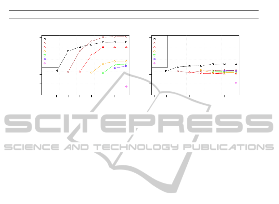
Table 4: Parameters for the Growing Neural Gas algorithm.
Parameter ε
b
ε
n
λ a
max
α d hold sup
value 0.05 0.005 250 1000 0.5 0.9 0.1 10%
0 1 2 3 4 5 6 7
0.03 0.05 0.07 0.09
Part 1
Part 2
Part 3
Part 4
Part 5
Part 6
Part 7
Steps
Average SSE
Quantization error
(a) Using GNG
0 1 2 3 4 5 6 7
0.03 0.05 0.07 0.09
Part 1
Part 2
Part 3
Part 4
Part 5
Part 6
Part 7
Steps
Average SSE
Quantization error
(b) Using GNG-m
Figure 13: Average quantization error for each one of the parts at each step.
the network has information of how many times the
unit has been selected as the nearest unit of any ob-
servation in the dataset. We call this information the
mass of the unit. In this way, units having a smaller
mass can move more easily than units having a larger
mass. The tests we performed showed how these new
parameters can be useful in alleviating the problem of
catastrophic forgetting in incremental learning.
However, these modifications to the algorithm do
not consider the possibility of building models from
data coming from dynamic systems. The GNG-m al-
gorithm can increase the property of memory, which
represents stability, but at the same time decreases the
plasticity of the network. Increasing stability is de-
sired in the case of modelling a large dataset because
catastrophic forgetting is undesirable. Conversely,
forgetting becomes an important feature when the
process generating the data changes over time. In this
case, a policy such as “mass-decay” can be a feasi-
ble approach to control the ability of the network to
forget the oldest events, and thus remaining plastic to
capture the changing dynamics of the process being
modelled.
REFERENCES
Bouchachia, A., Gabrys, B., and Sahel, Z. (2007).
Overview of some incremental learning algorithms. In
Proceedings of the Fuzzy Systems Conference, 2007.
FUZZ-IEEE 2007, pages 1–6.
Carpenter, G. A. and Grossberg, S. (1987). Art 2: self-
organization of stable category recognition codes for
analog input patterns. Appl. Opt., 26(23):4919–4930.
Chalup, S. K. (2002). Incremental learning in biological
and machine learning systems. Int. J. Neural Syst.,
12(6):447–465.
French, R. M. (1994). Catastrophic forgetting in connec-
tionist networks: Causes, consequences and solutions.
In Trends in Cognitive Sciences, pages 128–135.
Fritzke, B. (1995). A growing neural gas network learns
topologies. In Advances in Neural Information Pro-
cessing Systems 7, pages 625–632. MIT Press.
Fritzke, B. (1997). Unsupervised ontogenic networks. In
Handbook of Neural Computation, chapter C 2.4. In-
stitute of Physics and Oxford University Press.
Giraud-Carrier, C.(2000). A note on the utility of incremen-
tal learning. Aicommunications, 13(4):215–223(9).
Grossberg, S. (1987). Competitive learning: From interac-
tive activation to adaptive resonance. Cognitive Sci-
ence, 11(1):23 – 63.
Heinke, D. and Hamker, F. H. (1998). Comparing neural
networks: a benchmark on growing neural gas, grow-
ing cell structures, and fuzzy ARTMAP. IEEE Trans-
actions on Neural Networks, 9(6):1279–1291.
Hijmans, R. J., Cameron, S. E., Parra, J. L., Jones, P. G., and
Jarvis, A. (2005). Very high resolution interpolated
climate surfaces for global land areas. International
Journal of Climatology, 25(15):1965–1978.
McCloskey, M. and Cohen, N. J. (1989). Catastrophic in-
terference in connectionist networks: The sequential
learning problem. In Bower, G. H., editor, The Psy-
chology of Learning and Motivation: Advances in Re-
search and Theory, volume 24, pages 109–136. Aca-
demic Press inc.
Robins, A. (2004). Sequential learning in neural networks:
A review and a discussion of pseudorehearsal based
methods. Intell. Data Anal., 8(3):301–322.
Sarle, W. S. (2002). comp.ai.neural-nets faq - part 2. Avail-
able: http://www.faqs.org/faqs/ai-faq/neural-nets/part2/.
Satiz´abal, H. F., Perez-Uribe, A., and Tomassini, M. (2009).
Avoiding prototype proliferation in incremental vector
quantization of large heterogeneous datasets. In Con-
structive Neural Networks, pages 243–260. Springer
Berlin / Heidelberg.
NCTA 2011 - International Conference on Neural Computation Theory and Applications
276
