
FUNCTIONAL NETWORK IN NAVIGATION SATELLITE
CLOCK ERROR PREDICTION
A Novel Application
Ying Wang
1
, Bo Xu
1,2
and Xuhai Yang
3
1
College of Astronautics, Nanjing University of Aeronautics and Astronautics, Yudao street, Nanjing, China
2
School of Astronomy & Space Science, Nanjing University, Nanjing, China
3
National Time Service Centre, Xi’an, China
Keywords: Functional network, Time delay, Satellite clock error, Clock error prediction, Neural network.
Abstract: In order to describe the characteristics of navigation satellite clock error better and improve navigation
satellite clock error prediction accuracy, a satellite clock prediction method based on functional network is
proposed in this paper. The method added delay variables to the traditional functional network which can
reflect the dynamical characteristics of navigation satellite clock error better than the traditional method
without delay variables. The GPS satellites are taken for example; simulation results show that the
prediction accuracy of the proposed method is better than those of quadratic polynomial, quadratic
polynomial with periodic term, ARIMA and the grey methods.
1 INTRODUCTION
The performance of a navigation satellite are related
to the behaviour of the atomic clocks hosted on the
satellite; the real-time and reliable prediction of the
behaviour of such clocks is needed to provide
precise navigation performances and to optimize the
interval between uploading of the corrections to the
satellite clocks. Take Global Navigation Satellite
System (GNSS) for example, the IGS, along with a
multinational membership of organizations and
agencies, provides GPS orbits and clocks, tracking
data, and other high-quality GPS data and data
products online to meet the objectives of a wide
range of scientific and engineering applications and
studies. The accuracy of the satellite and station
clocks is announced to be better than 0.1 ns, while
the orbits’ accuracy to be less than 5
cm
(Delporte,
2004). In fact, these high-accuracy data are not
available in real time but a posteriori, with a delay
up to 13 days, while the broadcast ephemeris is
realized in real time which accuracy reaches 5
ns
.
Many papers have dealt with the prediction
problem. Zhang et al. (2007) constructed a model
which includes a quadratic polynomial and the
periodic terms. Cui and Jiao (2005) introduced the
grey system into the research on the prediction of the
clock error of the navigation satellite and obtained
better results. Xu and Zeng (2009) proposed a new
ARIMA (0, 2, q) model to predict the clock error
and gained a series of important achievements.
However, further studies show that there exist some
limitations in the classical methods of navigation
satellite clock error prediction. On the basis of
exploration of the limitations of the satellite clock
error prediction conducted by means of the
traditional models, we present a novel research on
the navigation satellite clock error prediction based
on functional network.
Castillo et al. (1999) introduced functional
network as a generalization of the standard neural
network. Unlike neural networks that are basically
driven by data, functional network may be
considered more as problem-driven models than as
data-driven models. Functional networks have been
successfully demonstrated in some sample
applications, e.g. to extract information masked by
chaos (Castillo and Gutierrez, 1998), and have been
used for nonlinear system identification (Li et al.,
2001). It has also been used for predicting fresh and
hardened properties of self-compacting concretes
(Tomasiello, 2011).
In this paper, we apply an alternative new
approach using functional networks in navigation
satellite clock error prediction. And, the results are
41
Wang Y., Xu B. and Yang X..
FUNCTIONAL NETWORK IN NAVIGATION SATELLITE CLOCK ERROR PREDICTION - A Novel Application.
DOI: 10.5220/0003680100410050
In Proceedings of the International Conference on Neural Computation Theory and Applications (NCTA-2011), pages 41-50
ISBN: 978-989-8425-84-3
Copyright
c
2011 SCITEPRESS (Science and Technology Publications, Lda.)

used to compare with the conventional grey method
(GM), the quadratic polynomial method (QPM), the
quadratic polynomial with periodic term method
(QPPTM) and the autoregressive integrated moving
average method (ARIMA). The paper is organized
as follows: Section 2 is a brief description of
functional network. The functional network used in
this study is demonstrated and its mathematical
representation is presented in detail. Section 3
describes the atomic clock error prediction model
based on functional network, while the mathematical
model of atomic clock error is combined with and
derived. Section 4, five separate tests were carried
out on the materials of the GPS satellite clock error
of 20 different and continuous time intervals. The
results are shown in Section 5, where the models’
ability to predict satellite atomic clock error at
different time intervals are compared. Some
diagrams from the simulation are presented in that
section. The final conclusions are presented in
Section 6.
2 FUNCTIONAL NETWORK
Figure 1 shows a typical architecture of a functional
network illustrating its main components. A
functional network consists of several elements
including: one layer of input storing neurons, one
layer of output storing neurons, one (or more) layers
of processing neurons, optional layers of
intermediate storing neurons, and a set of direct links
between them (Castillo, 1998).
(
)
112
,
f
xx
()
223
,
f
xx
()
345
,
f
xx
1
x
2
x
3
x
4
x
5
x
6
x
Figure 1: Functional network architecture.
A processing neuron receives a set of input
signals coming from the previous layer and delivers
the result of its calculation to the next layer
following the direction of the links. Each processing
neuron is associated with a function, which can be
multivariate and can have as many arguments as
there are inputs to the neuron. The input, output, or
intermediate information produced by processing
neurons is stored in storing neurons. The functions
associated with processing neurons are the key to
functional networks. Unlike artificial neural
networks, in functional networks, neuron functions
are unknown (arbitrary) functions from given
families that must be determined during the training
process. There are no weights in functional networks
as their function in ANN is now incorporated into
the neuron functions.
To work with functional networks, in addition to
the data information, it is important to understand
the problem to be solved since the selection of the
topology of a functional network is normally based
on the properties which usually lead to a clear and
single network structure. From the different possible
functional network forms, the separable functional
network is a simple family with many applications.
It uses a functional expression that combines the
separated efforts of input variables. In this study, our
goal is to predict atomic clock error using both the
current time and the atomic clock error at previous
time steps as inputs. The separable functional
network may be used as the approximate model in
atomic clock error prediction on the basis of the
physical model of the atomic clock.
2.1 Separable Functional Network
In this section, we demonstrate a simple separable
functional network with two inputs and one output.
Figure 2 depicts the topology of a separable
functional network. The relationship between
z ,
x
and
y can be defined mathematically as follows,
() ()()
1
,
n
ii
i
zFxy fxgy
=
==
∑
(1)
where
x
, y are the two input variables and z is the
output of the functional network.
()
i
f
⋅
,
(
)
i
g ⋅
are the
unknown neuron functions.
×
×
×
1
f
2
f
n
f
1
g
2
g
n
g
y
x
z
Figure 2: The general separable functional network
architecture.
2.2 The Uniqueness of Representation
Before using functional networks, it is important to
make sure of the uniqueness of the representation of
the network in order to obtain a more general set of
functions satisfying a given network topology. This
is due to the danger that, in some cases, different
neuron functions may lead to exactly the same
NCTA 2011 - International Conference on Neural Computation Theory and Applications
42

output for the same input thereby leading to an ill-
conditioned estimation problem (Bruen and Dooge,
1984). To address this problem, Castillo and
Gutierrez have given a general solution (Theorem 1)
for all the functional networks of Eq. (1) as follows:
Theorem 1. All solutions of equation
() ()
1
0
n
ii
i
fxgy
=
=
∑
can be written in the form
(
)
(
)
A
x
x=f
ϕ
,
(
)
(
)
Byy=g
ψ
, where A and B are
constant matrices (of dimensions
nr
×
and
(
)
nnr×− , respectively) with
T
0=AB , and
() () ()
()
1
,...,
r
x
xx
ϕϕ
=
ϕ
,
(
)
(
)
(
)
(
)
1
,...,
rn
yyy
ψψ
+
=
ψ
are two arbitrary systems of mutually linearly
independent functions, and
r is an integer between
0 and n .
It is important to notice that an initial value for the
neuron function(s) has to be assigned to represent
the uniqueness conditions.
In this study we start with the simplest network
structure by assuming
12
1gf
=
= with 2n = , Then,
Eq. (1) can be simplified to
(
)
(
)
(
)
,zFxy fx gy==+
(2)
2.3 Training
Training is an important stage in the application of a
functional network. It is also equivalent, in practice,
to the fitting process in conventional methods of
modelling. The process of training the functional
network associated with Eq. (2) is equivalent to
estimating the neuron functions
()
f
⋅
and
(
)
g
⋅
from
the available data. The objective is to minimize an
error function that measures the difference between
the model output
ˆ
z
and the actual (measured)
values
z .
From Theorem 1, we can approximate the neuron
functions by considering a linear independent
combination of a standard form for each neuron
function. The standard functional form
()
,
j
j
ϕ
ψ
can
be a polynomial family, a Fourier series, or any
other set of linearly independent functions.
Therefore, the neuron functions can be expressed as
() ()
1
ˆ
p
jj
j
f
xax
ϕ
=
=
∑
(3)
() ()
1
ˆ
q
jj
j
g
yby
ψ
=
=
∑
(4)
For a clearer presentation in the following
calculations, we use the same parameter symbols for
Eq. (3) and (4), and rewrite Eq. (4) as
() ()
1
ˆ
pq
jjp
jp
g
yay
ϕ
+
−
=+
=
∑
(5)
where the coefficients
j
a are the parameters of the
functional networks, and
p , q are the orders of
either the polynomial family or Fourier series. The
objective function used here is the sum of square
errors, which should be minimized,
() ()
2
2
11
ˆ
ˆ
ˆ
kk
ii i
ii
Qe zfxgy
==
⎡
⎤
== − −
⎣
⎦
∑∑
(6)
where k is the training sample size. For a unique
representation of the functional networks, we must
add an initial functional condition. In this case we
can use either of the two initial conditions,
(
)
0
f
xu
=
(7)
(
)
0
g
yv
=
(8)
where
0
x
,
0
y and u , v are given constants.
Therefore, we use Eq. (7) as a penalty term adding
to the objective function (Eq. (6)). Using a Lagrange
multiplier, Eq. (6) becomes
()
(
)
0
ˆ
QQ fx u
λ
λ
=
+−
(9)
where
λ
is a constant. Minimization of the above
function
Q
λ
is equivalent to solving the set of
derivative equations of
Q
λ
with respect to
parameters
j
a and multiplier
λ
.Then, we have
() () ()
()
11 1
0
2
0, 1,...,
ppq
k
ijji jjpiri
ij jp
r
r
Q
zax a y x
a
xr p
λ
ϕϕϕ
λϕ
+
−
== =+
⎡⎤
∂
=− − −
⎢⎥
∂
⎣⎦
+==
∑∑ ∑
(10)
() () ()
11 1
2
0, 1,...
ppq
k
ijji jjpirpi
ij jp
r
Q
zax a y y
a
rp pq
λ
ϕϕϕ
+
−−
== =+
⎡⎤
∂
=− − −
⎢⎥
∂
⎣⎦
==+ +
∑∑ ∑
(11)
()
0
1
0, 1,...
p
jj
j
Q
axur p
λ
ϕ
λ
=
∂
=−==
∂
∑
(12)
This leads to a system of 1pq++ linear equations
where the unknown coefficients are parameters
j
a
and
λ
.
FUNCTIONAL NETWORK IN NAVIGATION SATELLITE CLOCK ERROR PREDICTION - A Novel Application
43

3 THE CLOCK ERROR
PREDICTION MODEL BASED
ON FUNCTIONAL NETWORK
3.1 The Mathematical Model of Atomic
Clock Error
The clock signal is typically affected by five random
noises that are known in metrological literature as
white phase noise (WPN), flicker phase noise (FPN),
white frequency noise (WFN) that produces a
Brownian motion (BM) (also called Wiener process
or random walk) on the phase, flicker frequency
noise (FFN) and random white frequency noise
(RWFN), which produces an integrated Brownian
motion (IBM) on the phase. The presence of
different kinds of random noises and their entity is
different from clock to clock. From experimental
evidence it appears that on the caesium clock the
predominant noises are the WFN and the RWFN
that correspond in mathematical language to the
Wiener process and to the integrated Wiener
process, respectively, on the phase deviation.
Denoting by
(
)
1
X
t the atomic clock phase deviation,
its time evolution can be written as a dynamical
system of stochastic differential equation as (Panfilo
and Tavella, 2008)
() () ()
() ()
12 11
222
ddd,
ddd
X
tXtt Wt
Xt d t Wt
σ
σ
⎧
=⋅+
⎪
⎨
=⋅ +
⎪
⎩
(13)
with initial conditions
(
)
(
)
102 0
0,0
X
xX y==, which
represent the initial phase and frequency deviation.
The constant
d indicates the frequency aging or
drift. The triplet
(
)
00
,,
x
yd represents what is
generally referred to as the deterministic phenomena
of the atomic clocks. The positive constants
1
σ
and
2
σ
represent the diffusion coefficients of the two
noise components
1
W and
2
W , while indicate the
intensity of each noise.
()
1
Wt
is the Wiener noise
acting on the phase deviation
1
X
and corresponding
to a WFN; the Wiener process can, in fact, be
thought of as the integral of a white noise.
(
)
2
Wt
represents the Wiener process acting on the
frequency (the so-called ‘random walk FN’) and
yields to an integrated Wiener process on the phase.
The Wiener process
(
)
{
}
,0Wt t≥ is defined as a
Gaussian process that starts from
(
)
{
}
00W
=
and
then at any instant has a probability distribution
given by
(
)
0,
N
t with a zero mean value and
variance equal to
t .
Note that
1
X
represents the phase deviation,
while the frequency deviation results in
1
X
. The
second component
2
X
is only a part of the clock
frequency deviation, i.e. what is generally called the
‘random walk’ frequency component.
Since Eq. (13) is a complete strictly linear
stochastic differential equation, it is possible to
obtain its solution in closed form as
() () ()
() ()
2
100 11 22
0
20 22
d,
2
.
t
t
X
txytd Wt Wss
Xt y dt Wt
σσ
σ
⎧
=+ +⋅+ +
⎪
⎨
⎪
=+⋅+
⎩
∫
(14)
Let us now consider a fixed time interval 'T and an
equally spaced partition
01
0'
N
tt t T≡<< < ≡ and
let us denote the resulting discretization step
with
1kk
tt
τ
+
=
− , for each 0,1,..., 1kN=−. We can
express solution Eq. (14) at epoch
1k
t
+
in terms of
the process at epoch
k
t as
( ) () ()
()
2
11 1 2 ,1
21 2 ,2
,
2
() .
kkk k
kk k
X
tXtXtd J
Xt Xt d J
τ
τ
τ
+
+
⎧
=+ +⋅+
⎪
⎨
⎪
=+⋅+
⎩
(15)
where the vector
k
J
is normally distributed as
32
22 2
12 2
2
22
22
32
,.
2
0
k
N
ττ
στ σ σ
τ
σστ
⎛⎞
⎡
⎤
+
⎜⎟
⎢
⎥
⎜⎟
⎢
⎥
⎜⎟
⎢
⎥
⎜⎟
⎢
⎥
⎣
⎦
⎝⎠
∼J
(16)
The measured values of atomic clock error
(
)
1k
X
t
+
is
(
)
(
)
(
)
() () ()
111 1
2
12 ,11
2
kkk
kk kk
Xt X t t
Xt Xt d J t
ε
τ
τε
+++
+
=+
=+ +⋅++
(17)
where
(
)
t
ε
is the Gaussian measurement noise
with
(
)
(
)
2
0,tN
ε
σ
∼ . Finally, the mathematical
model of atomic clock error can be written as
( ) () () ()
1
2
12
d
2
k
k
t
kkk
t
X
tXtXtd ftt
τ
τ
+
+
=+ +⋅+
∫
(18)
where
1kk
tt
τ
+
=
− ,
(
)
1k
X
t
+
is the navigation satellite
clock error at the time of
1k
t
+
,
()
k
X
t is the satellite
clock error at the referent time of
k
t ,
()
2 k
X
t is the
frequency deviation of clock at the referent time of
k
t , d is the frequency aging or drift of clock at the
NCTA 2011 - International Conference on Neural Computation Theory and Applications
44

referent time of
k
t and
()
1
d
k
k
t
t
f
tt
+
∫
is a kind of
random clock error caused by the random error of
frequency, of which the statistical characteristics can
be described only through the degree of stability of
the clock and the concrete value can not be known.
Since the traditional QPM neglects the stochastic
component during the clock error model building,
and the GM can not make full use of existing clock
error data, the identification of the ARIMA is
relatively difficult. Thus the precision of clock error
prediction of these traditional models is low.
According to the present research situations, we
apply functional network in navigation satellite
clock error prediction, while both the trend item and
the stochastic component of the atomic clock error
are considered comprehensively.
3.2 The Clock Error Prediction Model
based on Functional Network
In this paper we use both the current time and the
atomic clock error at previous time steps as inputs,
and use the current clock error as output of the
prediction model. This method of modelling makes
the functional network fully study the dynamic
characteristic of the historical data of the clock error,
and avoid the disadvantage of QPM, which is the
error accumulation become more and more obvious
with the lapse of time, while QPM simply uses time
as input. Figure 3 shows the structure of the model
of the train stage.
()
k
x
t
(
)
ˆ
k
X
t
k
t
(
)
k
yt
(
)
k
t
ε
(
)
k
X
t
k
t
(
)
(
)
1
,...,
kkd
Xt Xt
−−
+
+
+
−
Figure 3: Diagram of satellite clock error train structure
based on functional network.
where
k
t represents current time,
()
k
yt represents
the navigation satellite clock error at current time,
()
k
t
ε
is the measurement error,
()
k
X
t represent the
actual observed value of the clock error at current
time,
(
)
(
)
1
,...,
kkd
Xt Xt
−−
represent the clock errors at
previous time steps. The inputs of functional
network are
k
t and
(
)
(
)
1
,...,
kkd
Xt Xt
−−
, the output
is
()
ˆ
k
X
t , which is the prediction value of clock error
at current time,
(
)
k
x
t
is the prediction error at
current time. During the training process, the
functional network approximates the functional
relationship expressed as:
(
)
(
)
(
)
(
)
() ( )
1
1
ˆ
, ,...,
ˆ
ˆ
kkk kd
d
tktk
k
Xt Ft Xt Xt
ft f x
−−
−
=
=
=+
∑
(19)
where
(
)
ˆ
t
f
t , which is the contribution of current
time, denotes the trend item, and
()
1
ˆ
d
ktk
k
fx
−
=
∑
, which
is the combination of the contributions of the clock
errors at previous time steps, denotes the stochastic
component of the atomic clock error.
We adopt the method of non-mechanism
modelling, using current time and history data of
clock error and high non-linear mapping of
functional network, the input-output relationship of
practical system of the atomic clock error is
simulated and the model which has been set by
training can be used in the prediction stage, the
structure of the model of this stage is shown in
Figure 4.
(
)
(
)
1
ˆˆ
,...,
kkd
Xt Xt
−−
(
)
ˆ
x
k
(
)
tk
Figure 4: Diagram of satellite clock error prediction
structure based on functional network.
Considering the mathematical model of atomic
clock error, we choose the polynomial family for the
standard functional form
(
)
,
j
j
ϕ
ψ
. In addition, an
initial condition function
(
)
0
f
xu= is assigned in
order to obtain the unique representation.
4 APPLICATION TO
NAVIGATION SATELLITE
CLOCK ERROR PREDICTION
In order to verify the feasibility and effectiveness of
this method, we carried out five separate tests on the
clock error prediction, and compared its
performance with the other four conventional
methods, which are the GM, QPM, QPPTM and
ARIMA. To ensure obtaining reliable model
comparisons, we used the GPS satellite clock error
of 20 different and continuous time intervals for
each test, and the materials of the GPS clock error,
which were used in the tests, are the precise satellite
clock solutions published by IGS with five minutes
sampling interval. For the data pre-process,
FUNCTIONAL NETWORK IN NAVIGATION SATELLITE CLOCK ERROR PREDICTION - A Novel Application
45

according to the anomalies and missing values of the
atomic clock error, firstly we performed integrity
check on the data, and then adopted Baarda data
detection method in anomaly detection, finally used
Lagrange interpolation interpolates these data after
the anomalies removal.
The available data for each test was divided into
two groups: training (calibration) set
A
, and testing
(validation) set
B
. The GM, QPM, QPPTM,
ARIMA and FN were fitted to the calibration data,
where the GM adopted the same modelling scheme
as Cui and Jiao (2005), which used the 8 initial
epochs before the prediction time for modelling; The
QPPTM reduced the noise of the residuals on the
basis of quadratic fitting, which was realized by
utilizing the spectrum analysis; The ARIMA
model’s order determination was completed by
Bayesian information criterion (BIC). As for the FN
model, due to the dynamic characteristic of clock
error of different satellite is not the same at the
different time interval, to make precisely prediction,
we chose a set of candidate networks, with the num
of input nodes from 2 to 5, and the num of basis
functions which combine the processing neuron of
FN from 2 to 5, here once again the calibration set
A
was divided into two groups: training
(calibration) set
A
′
and testing (validation) set
B
′
.
The candidate model structures were fitted to the
calibration data
A
′
, and were predicted to the
validation data
B
′
; the best performing model from
them was selected to represent them, and would be
fitted to the calibration set
A
, which was the same
step as others.
Five separate simulation prediction tests were
carried out; the simulation results would be given in
diagrams. Considering that different kinds of atomic
clock onboard may have differences, both the
figures of error curve of PRN10 and PRN11 were
given, of which both the start time of prediction is
January 8, 2009, where PRN10 is the satellite
equipped with the caesium clock and PRN11 is the
satellite equipped with the rubidium clock. In
addition, the average values of prediction errors of
each satellite of 20 different time intervals would be
given, and discussions would be carried out
according to different kinds of atomic clocks
onboard. The concrete contents of tests are as
follows.
Test 1: 6 hours prediction test was carried out,
adopting the above five methods and utilizing the
GPS satellite clock error of 20 different and
continuous time intervals. The time interval of
simulation spanned from January 7 to 11, 2009. The
simulation results was shown in Figure 5, and the
average values of prediction errors of each satellite
of 20 different time intervals, which were obtained
by five methods is summarized in Table 1.
Test 2: 12 hours prediction test was carried out,
adopting the above five methods and utilizing the
GPS satellite clock error of 20 different and
continuous time intervals. The time interval of
simulation spanned from January 7 to 16, 2009. The
simulation results was shown in Figure 6, and the
average values of prediction errors of each satellite
of 20 different time intervals, which were obtained
by five methods is summarized in Table 2.
Test 3: 1 day prediction test was carried out,
adopting the above five methods and utilizing the
GPS satellite clock error of 20 different and
continuous time intervals. The time interval of
simulation spanned from January 7 to 27, 2009. The
simulation results was shown in Figure 7, and the
average values of prediction errors of each satellite
of 20 different time intervals, which were obtained
by five methods is summarized in Table 3.
Test 4: 7 days prediction test was carried out,
adopting the above five methods and utilizing the
GPS satellite clock error of 20 different and
continuous time intervals. The time interval of
simulation spanned from January 7 to February 2,
2009. The simulation results was shown in Figure 8,
and the average values of prediction errors of each
satellite of 20 different time intervals, which were
obtained by five methods is summarized in Table 4.
Test 5: 14 days prediction test was carried out,
adopting the above five methods and utilizing the
GPS satellite clock error of 20 different and
continuous time intervals. The time interval of
simulation spanned from January 7 to February 9,
2009. The simulation results was shown in Figure 9,
and the average values of prediction errors of each
satellite of 20 different time intervals, which were
obtained by five methods is summarized in Table 5.
5 RESULTS AND DISCUSSIONS
For the test 1 (6 hours prediction), Table 1
demonstrates the performances of the five methods
in terms of average errors of 20 different time
interval, since the QPM can make full use of
existing clock error data, which has a good reflection
of the whole change rule of the clock error, the
prediction precision of which is equivalent with the
GM’s except PRN27. The QPPTM considers the
characteristics of the periodical changes on the basis
of the QPM, so the prediction precision is better than
the latter’s. The prediction precision of functional
NCTA 2011 - International Conference on Neural Computation Theory and Applications
46

network is superior to those of the other four
methods’, except that the prediction precision of
PRN11 and PRN24 are equivalent with the others.
For the test 2 and test 3 (12 hours prediction and
1 day prediction), the prediction precisions of the
QPM and the QPPTM are overall superior to that of
the GM. Due to the identification of the ARIMA is
relatively difficult, the prediction performance of
ARIMA is unstable, where the optimal prediction
precision of the ARIMA for 12 hours prediction is
0.8
ns , while the poorest can reach up to the order
of
s
μ
. The prediction precision of functional
network is superior to those of the other four
methods’, except that the prediction precisions of
PRN 28 in 12 hours prediction and PRN32 in 1 day
prediction are equivalent with the others.
For the test 4 (7 days prediction), compared with
the other four methods, the prediction precision of
functional network totally has improvement, with
the average values of the prediction error is 0.4
percent of other methods’ under the best situation,
and 95.2 percent of other methods’ under the poorest
situation of improvement.
For the test 5 (14 days prediction), the analysis of
the prediction precision between that of the QPM
and the GM displays that owing to the
characteristics of the error accumulation of the
QPM, with the increase in the prediction time, the
prediction precision of the GM is evidently superior
to that of the QPM. Due to the influence of the
QPM, which is the principle term, the QPPTM also
shows the characteristics of the error accumulation,
with slightly better than the QPM. The prediction
precision of functional network totally has
improvement compared with the other four
methods’, with the average values of the prediction
error is 0.2 percent of other methods’ under the best
situation, and 93.6 percent of other methods’ under
the poorest situation of improvement.
1513.71 1513.72 1513.73 1513.74 1513.75
-5
0
5
10
15
20
25
30
Prediction error/ns
Epoch/wee
k
Test 1: 6 hours prediction
GM
QPM
QPPTM
ARIMA
FN
GM
QPM
QPPTM
ARIMA
FN
Figure 5(a): 6 Hours prediction error of PRN10.
1513.71 1513.72 1513.73 1513.74 1513.75
-1
-0.5
0
0.5
1
1.5
2
2.5
Prediction error/ns
Epoch/week
Test 1: 6 hours prediction
GM
QPM
QPPTM
ARIMA
FN
GM
QPM
QPPTM
ARIMA
FN
Figure 5(b): 6 Hours prediction error of PRN11.
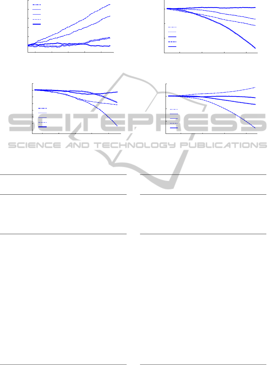
From all the tests above, we can see that the
prediction precision of functional network totally
has improvement compared with the other four
methods’, especially for the test 4 and test 5, which
are 7 days and 14 days prediction tests. In addition,
the prediction precisions of the rubidium clock are
superior to the caesium clock, which is true for all
the methods in the five tests.
Table 1: Comparison among the 6 hours prediction
accuracy (unit: ).
Kind of
clock
onboard
PRN GM QP QPPTM ARIMA FN
Caesium
clock
03 5.14 5.07 5.00 10.0 4.78
09 4.88 6.57 6.21 10.4 4.40
10 7.30 4.12 3.98 47.6 3.20
24 5.33 6.21 6.19 6.67 8.77
27 7.38 16.80 16.7 16.5 9.71
30 8.09 8.29 8.22 9.98 4.17
Rubidium
clock
02 0.73 0.59 0.58 1.75 0.34
04 1.81 1.78 1.77 13.4 1.21
07 0.70 0.83 1.11 1.06 0.56
11 0.68 0.64 0.63 0.66 0.70
12 1.08 1.62 1.59 1.93 0.63
13 0.88 0.88 0.87 1.22 0.52
14 0.77 0.83 0.81 2.91 0.43
15 1.09 0.58 0.57 4.05 1.01
16 1.06 1.41 1.37 3.11 0.68
17 0.92 0.38 0.37 1.82 0.33
18 0.98 0.86 0.84 1.79 0.52
19 0.75 0.64 0.63 0.91 0.36
20 1.17 1.09 1.08 1.74 0.35
21 1.24 0.97 0.94 1.58 0.58
22 2.35 1.21 1.20 1.18 0.65
23 0.67 0.56 0.54 0.93 0.28
28 0.93 0.97 0.96 66.6 0.63
29 0.67 0.71 0.70 1.10 0.37
31 0.63 0.73 0.71 1.42 0.45
32 1.45 3.53 3.51 4.56 1.83
ns
FUNCTIONAL NETWORK IN NAVIGATION SATELLITE CLOCK ERROR PREDICTION - A Novel Application
47

1513.71 1513.73 1513.75 1513.77 1513.79
-10
0
10
20
30
40
Prediction error/ns
Epoch/week
Test 2: 12 hours prediction
GM
QPM
QPPTM
ARIMA
FN
GM
QPM
QPPTM
ARIMA
FN
Figure 6(a): 12 Hours prediction error of PRN10.
1513.71 1513.73 1513.75 1513.77 1513.79
-8
-6
-4
-2
0
2
Prediction error/ns
Epoch/week
Test 2: 12 hours prediction
GM
ARIMA
FN
QPM
QPPTM
GM
QPM
QPPTM
ARIMA
FN
Figure 6(b): 12 Hours prediction error of PRN11.
Table 2: Comparison among the 12 hours prediction
accuracy (unit: ).
Kind of
clock
onboard
PRN GM QP QPPTM ARIMA FN
Caesium
clock
03 10.6 11.4 11.3 7.52 5.25
09 11.2 15.7 15.6 13.7 7.05
10 12.6 8.31 8.27 9.69 5.90
24 9.71 9.84 9.78 777 4.49
27 18.7 27.0 26.7 50.5 8.25
30 17.6 16.1 16.0 452 6.48
Rubidium
cloc
02 1.77 1.34 1.35 0.81 0.47
04 3.69 4.23 4.22 16.2 1.50
07 1.26 0.95 0.94 1.08 0.51
11 1.35 2.66 2.65 2.28 0.39
12 1.82 2.33 2.31 1.93 0.53
13 1.39 1.56 1.55 1.84 0.60
14 1.53 0.90 0.87 2.86 0.51
15 1.41 1.23 1.22 3.99 1.01
16 1.51 1.83 1.80 2.32 0.37
17 2.03 1.17 1.16 1.09 0.43
18 2.05 1.02 1.00 2.86 0.44
19 1.43 1.21 1.19 1.44 0.44
20 2.10 1.16 1.14 1.85 0.55
21 2.57 1.61 1.60 1.98 0.62
22 3.57 1.46 1.44 1.11 0.89
23 1.66 0.75 0.73 0.87 0.37
28 2.01 1.91 1.90 110 2.03
29 1.08 1.08 1.07 1.39 0.61
31 1.37 1.47 1.47 2.29 0.64
32 3.21 3.45 3.39 10.4 1.96
1513.72 1513.76 1513.8 1513.84
-20
-10
0
10
20
30
40
50
Prediction error/n
s
Epoch/week
GM
QPM
QPPTM
ARIMA
FN
Test 3: 1 day prediction
GM
QPM
QPPTM
ARIMA
FN
Figure 7(a): 1 Day prediction error of PRN10.
1513.72 1513.76 1513.8 1513.84
-2
-1
0
1
2
3
4
Prediction error/ns
Epoch/week
GM
QPM
QPPTM
ARIMA
FN
Test 3: 1 day prediction
GM
QPM
QPPTM
ARIMA
FN
Figure 7(b): 1 Day prediction error of PRN11.
Table 3: Comparison among the 1 day prediction accuracy
(unit: ).
Kind of
clock
onboard
PRN GM QP QPPTM ARIMA FN
Caesium
clock
03 22.7 13.1 13.0 15.5 6.38
09 21.37 15.38 15.32 99.7 8.23
10 16.5 12.9 12.8 13.0 6.98
24 24.4 13.0 12.9 8128 5.98
27 34.7 15.8 15.4 41.3 14.9
30 26.81 14.2 14.1 6196 7.52
Rubidium
clock
02 3.29 1.33 1.32 1.69 0.64
04 6.26 3.31 3.20 20.8 1.72
07 2.80 1.79 1.78 1.55 0.90
11 2.88 0.95 0.94 3.02 1.33
12 2.97 1.22 1.20 2.93 0.58
13 2.77 1.63 1.60 2.43 0.85
14 3.30 1.37 1.36 4.56 0.82
15 3.02 1.94 1.93 17.7 1.53
16 4.89 0.74 0.68 7.05 0.56
17 3.40 1.70 1.69 2.52 1.34
18 3.24 0.94 0.92 3.96 0.54
19 2.49 1.56 1.55 1.80 0.79
20 4.54 1.64 1.60 2.67 0.66
21 8.36 1.50 1.49 2.17 0.75
22 5.61 3.13 3.12 3.31 2.33
23 2.86 0.91 0.90 1.43 0.66
28 5.01 5.50 5.48 4.64 4.90
29 2.42 2.00 1.98 3.56 1.39
31 2.86 2.26 2.26 2.74 1.39
32 5.19 2.44 2.40 20.49 2.66
ns
ns
NCTA 2011 - International Conference on Neural Computation Theory and Applications
48
1513.8 1514 1514.2 1514.4 1514.6
0
100
200
300
400
500
Prediction error/ns
Epoch/week
QPM
QPPTM
ARIMA
FN
GM
Test 4: 7 days prediction
GM
QPM
QPPTM
ARIMA
FN
Figure 8(a): 7 Days prediction error of PRN10.
1513.8 1514 1514.2 1514.4 1514.6
-120
-100
-80
-60
-40
-20
0
20
Prediction error/ns
Epoch/week
GM
QPM
QPPTM
ARIMA
FN
Test 4: 7 days prediction
GM
QPM
QPPTM
ARIMA
FN
Figure 8(b): 7 Days prediction error of PRN11.
Table 4: Comparison among the 7 days prediction
accuracy (unit: ).
Kind of
clock
onboard
PRN GM QP QPPTM ARIMA FN
Caesium
clock
03 150.5 290.6 290.9 227.1 27.65
09 146.6 308.9 309.0 2118 37.51
10 127.2 223.2 220.2 283.7 28.80
24 172.4 251.4 250.9 804 27.8
27 275 334 330 852 33.0
30 176 313 312 504 30.53
Rubidium
clock
02 22.7 29.1 29.1 3112 11.5
04 49.4 70.6 70.4 462 19.2
07 20.9 38.7 38.6 35.7 8.36
11 20.5 26.8 26.7 47.9 10.7
12 25.8 22.4 21.4 50.2 8.51
13 20.4 35.7 35.4 38.1 5.71
14 32.8 27.9 27.2 39.8 5.85
15 24.8 41.0 40.0 352 9.09
16 30.5 14.5 14.4 66.2 5.01
17 29.7 40.3 40.4 635 17.8
18 23.1 21.1 21.0 89.3 3.79
19 18.8 30.3 30.2 23.7 4.86
20 31.5 36.7 36.2 38.2 5.81
21 54.2 28.2 28.0 39.8 5.28
22 50.9 78.2 78.0 67.9 34.2
23 20.0 15.3 14.8 17.0 5.06
28 31.2 123 121 859 29.7
29 36.6 33.6 33.4 156 20.1
31 20.74 54.11 40.85 60.09 12.99
32 33.30 41.23 40.80 412.7 23.66
1514 1514.5 1515 1515.5
-1500
-1000
-500
0
Prediction error/ns
Epoch/week
GM
QPM
QPPTM
ARIMA
FN
Test 5: 14 days prediction
GM
QPM
QPPTM
ARIMA
FN
Figure 9(a): 14 Days prediction error of PRN10.
1514 1514.5 1515 1515.5
-600
-400
-200
0
200
Prediction error/n
s
Epoch/week
GM
QPM
QPPTM
ARIMA
FN
Test 5: 14 days prediction
GM
QPM
QPPTM
ARIMA
FN
Figure 9(b): 14 Days prediction error of PRN11.
Table 5: Comparison among the 14 days prediction
accuracy (unit: ).
Kind of
clock
onboard
PRN GM QP QPPTM ARIMA FN
Caesium
clock
03 295.7 1058 1059 1e+4 71.46
09 304.9 1108 1108 2e+4 83.66
10 264 824 823 4e+5 49.1
24 350 914 912 8e+3 59.6
27 659 1201 1195 4e+5 62.8
30 355 1140 1132 3e+5 77.4
Rubidium
clock
02 52.49 107.5 107.6 4e+3 44.19
04 115 254 250 1e+3 11.0
07 44.6 139 139 206 20.7
11 46.1 106 106 351 23.7
12 69.8 80.7 80.5 301 38.1
13 43.8 131 130 166 13.9
14 92.6 102 101 309 18.8
15 73.6 143 141 2e+3 34.4
16 56.9 51.7 51.0 448 16.4
17 62.9 138 135 596 36.8
18 50.1 77.1 76.5 300 11.0
19 39.6 107 106 119 13.7
20 64.1 137.7 137.0 3e+4 17.2
21 104.0 102.5 102.0 154.8 14.92
22 96.2 269 265 292 69.9
23 41.8 54.3 54.1 137 16.8
28 58.1 463 460 3e+4 54.4
29 142 110 109 254 55.1
31 39.6 198 136 211 29.2
32 64.4 149 140 9e+4 57.4
ns
ns
FUNCTIONAL NETWORK IN NAVIGATION SATELLITE CLOCK ERROR PREDICTION - A Novel Application
49

6 CONCLUSIONS
Functional network is considered as a generalization
of artificial neural network, it is first introduced in
the problem of clock error prediction, and delay
variables are added to the traditional functional
network. In this study, five separate simulation tests
of the navigation satellite clock error prediction were
carried out, and five models were applied to it, using
the precise satellite clock solutions published by IGS
with five minutes sampling interval as simulation
data. The results of the simulation tests demonstrate
that the functional network, which is added with
delay variables, can reflect the dynamic
characteristics of navigation satellite clock error
better than the GM, QPM, QPPTM and ARIMA, as
the prediction precision is better than the others, and
can be used as a novel method in navigation satellite
clock error prediction.
ACKNOWLEDGEMENTS
This work was supported by the National Science
Foundation of China, 11078001 and 11033004.
REFERENCES
Bruen, M., Dooge, J. C. I., 1984. An efficient and robust
method for estimating unit hydrograph ordinates.
Journal of Hydrology, vol.70, February, pp.1-24.
Castillo, E., 1998. Functional Networks.
Neural
Processing Letters
, 7, pp. 151-159.
Castillo, E., Cobo. A., Gutiérrez J. M. et al., 1999.
Functional networks with applications: a neural-based
paradigm
. Boston et al.: Kluwer Academic Publishers.
Castillo, E., Gutiérrez, J. M., 1998. Nonlinear time series
modeling and prediction using functional networks.
Extracting information masked by chaos.
Physics
Letters A,
244, pp.71-84.
Cui X. Q., Jiao W. H., 2005. Grey system model for the
satellite clock error predicting.
Geomatics and
Information Science of Wuhan University
, vol. 30, no.
5, May, pp.447-450.
Delporte, J., 2004. Performance of GPS on board clocks
computed by IGS,
Frequency and Time Forum. EFTF
2004.18
th
European, Guildford, pp.201-207.
Li C. G., Liao X. F., He S. B. et al., 2001. Functional
network method for the identification of nonlinear
system.
System Engineering and Electronics, vol. 23,
no. 11, pp.50-53.
Panfilo, G., Tavella, P., 2008. Atomic clock prediction
based on stochastic differential equations.
Metrologia
45
, vol.45, no.6, December, pp.108-110.
Tomasiello, S., 2011. A functional network to predict
fresh and hardened properties of self-compacting
concretes.
International Journal for Numerical
Methods in Biomedical Engineering,
vol. 27, no.6,
June, pp.840-847.
Xu J. Y., Zeng A.M., 2009. Application of ARIMA(0,2,q)
model to prediction of satellite clock error.
Journal of
Geodesy and Geodynamics
, vol. 29, no. 5, October,
pp.116-120.
Zhang B., Ou J. K., Yuan Y. B. et al., 2007. Fitting
method for GPS satellite Clock errors using wavelet
and spectrum analysis.
Geomatics and Information
Science of Wuhan University
, vol.32, no.8, August,
pp.715-718.
NCTA 2011 - International Conference on Neural Computation Theory and Applications
50
