
ON THE ABSOLUTE VALUE OF TRAPEZOIDAL FUZZY NUMBERS
AND THE MANHATTAN DISTANCE OF FUZZY VECTORS
Julio Rojas-Mora
UMR ESPACE 6012 CNRS, Universit
´
e d’Avignon (UAPV), Avignon, France
Jaime Gil-Lafuente
Dept. of Business Economics and Organization, University of Barcelona, Barcelona, Spain
Didier Josselin
UMR ESPACE 6012 CNRS, Universit
´
e d’Avignon (UAPV), Avignon, France
Keywords:
Fuzzy sets, Manhattan distance, Absolute value.
Abstract:
The computation of the Manhattan distance for fuzzy vectors composed of trapezoidal fuzzy numbers (TrFN)
requires the application of the absolute value to the differences between components. The membership func-
tion of the absolute value of a fuzzy number has been defined by Dubois and Prade as well as by Chen and
Wang. The first one only removes the negative values of the fuzzy number, increasing its expected value.
Conversely, Chen and Wang’s definition maintains the expected value, but can produce a TrFN with negative
values. In this paper, we present the “positive correction” of the absolute value, a method to remove the nega-
tive values of a TrFN while maintaining its expected value. This operation also complies with a logic principle
of any uncertain distance: reducing the distance should also reduce its uncertainty.
1 INTRODUCTION
In several fields, the necessity to determine the dis-
tance that separates two points in
n
arises. When
there is uncertainty on the location of these points,
the calculation of the distance has to take this uncer-
tainty into consideration. By modeling uncertainty
with fuzzy subsets (Zadeh, 1965), it is possible to cal-
culate some form of distance that complies with this
consideration.
The literature is broad in this area, but a non-
comprehensive list of publications has to include the
work of (Voxman, 1998), who calculated crisp met-
rics between two fuzzy numbers, but who also ques-
tioned this approach, studying fuzzy distances be-
tween them. (Tran and Duckstein, 2002), in the con-
text of fuzzy numbers’ ranking, proposed a distance
function that takes into account all points in the fuzzy
numbers compared. (Chen and Wang, 2008) defined
a fuzzy distance that uses the absolute value of a
fuzzy number, calculated through its graded mean in-
tegration representation (GMIR). Finally, (Li and Liu,
2008) make use of an expected value operator to de-
fine a metric space of fuzzy variables.
In this paper, we will go back to the simplest rep-
resentation of the distance between two points, the
Manhattan distance. Applying this distance to trape-
zoidal fuzzy numbers (TrFN), we would like to obtain
a fuzzy number as a result, reflecting the uncertainty
on the distance itself. Nonetheless, we will subject
this distance to some conditions. Firstly, when the
distance is reduced, so must do its uncertainty. By
this, we mean that the uncertainty we have while as-
sessing a distance of about 20 Km has to be much
bigger that the uncertainty assessing a distance of 5
cm.
Secondly, the distance has to be positive at all
times, as a negative distance has no sense in the real
world. Finally, because we will be operating with
TrFN, we would like that the distance is also a TrFN.
For the calculation of the Manhattan distance be-
tween two fuzzy numbers, there is the need to define
the absolute value of a fuzzy number. We will ex-
plore the approaches followed by (Dubois and Prade,
399
Rojas-Mora J., Gil-Lafuente J. and Josselin D..
ON THE ABSOLUTE VALUE OF TRAPEZOIDAL FUZZY NUMBERS AND THE MANHATTAN DISTANCE OF FUZZY VECTORS.
DOI: 10.5220/0003674203990406
In Proceedings of the International Conference on Evolutionary Computation Theory and Applications (FCTA-2011), pages 399-406
ISBN: 978-989-8425-83-6
Copyright
c
2011 SCITEPRESS (Science and Technology Publications, Lda.)

1979) and (Chen and Wang, 2008), analyzing their
shortcomings according to the conditions previously
posed and proposing a solution that takes them into
consideration.
This paper introduces the basic concepts of fuzzy
sets and fuzzy numbers in Section 2. Then, on Sec-
tion 3, we will study the Manhattan distance as well
as the definitions of the absolute value for fuzzy num-
bers previously cited. Section 4 explains the proce-
dure needed to overcome the problems that arise from
the use of the absolute value according to our con-
straints. Finally, on Section 5 we will present the con-
clusions of this work.
2 FUZZY SUBSETS AND FUZZY
NUMBERS
In this section, we will introduce the basic definitions
use throughout this paper. We will start by defining
what a fuzzy subset is and what properties we will
ask of them.
Definition 1. A fuzzy subset
˜
F is a set whose elements
may not follow the law of excluded middle that rules
over Boolean logic, i.e., their membership function
can be mapped as:
µ
˜
F
: X → [0, 1].
In general, a fuzzy subset
˜
F can be represented
by a set of pairs consistent of the elements x of the
universal set X and a grade of membership µ
˜
A
(x):
˜
F =
{
(x, µ
˜
F
(x)) | x ∈ X , µ
˜
F
(x) ∈ [0, 1]
}
. (1)
Definition 2. An α-cut of a fuzzy subset
˜
F is defined
by:
F
α
= {x ∈ X : µ
˜
F
(x) ≥ α} , (2)
i.e., the subset of all elements that belong to
˜
F at least
in a degree α.
Definition 3. A fuzzy subset
˜
F is convex, if and only
if:
λx
1
+ (1 − λx
2
) ∈ F
α
∀x
1
, x
2
∈ F
α
, α, λ ∈ [0, 1], (3)
i.e., all the points in [x
1
, x
2
] must belong to A
α
, for any
α.
Definition 4. A fuzzy subset is “normal” if and only
if
max
x∈X
(µ
˜
F
(x)) = 1. (4)
Definition 5. The “core” of a normal fuzzy subset is:
N
˜
F
=
{
x : µ
˜
F
(x) = 1
}
. (5)
Now, we will define a fuzzy number based on
these definitions.
Definition 6. A fuzzy number M
e
is a convex, normal
fuzzy subset with domain in , for which:
1. ¯x := N
M
e
, card ( ¯x) = 1, and
2. µ
M
e
is, at least, piecewise continuous.
The first condition is usually dropped as there is a ten-
dency, that we will follow, to call “fuzzy numbers”
those fuzzy subsets for which the core has more than
one element (Zimmermann, 2005, 57).
Definition 7. A TrFN is defined by the membership
function:
µ
M
e
(x) =
1 −
x
2
−x
x
2
−x
1
, if x
1
≤ x < x
2
1, if x
2
≤ x ≤ x
3
1 −
x−x
3
x
4
−x
3
, if x
3
< x ≤ x
4
0 otherwise.
(6)
A TrFN is represented by a 4-tuple whose first
and fourth elements correspond to the extremes from
where the membership function begins to grow, and
whose second and third components are the limits of
the interval where the maximum certainty lies, i.e.,
M
e
= (x
1
, x
2
, x
3
, x
4
). From this point on, and for eas-
iness while operating with several TrFN’s, we will
change the “x” in the 4-tuple for the lowercase letter
that names a TrFN, i.e., M
e
= (m
1
, m
2
, m
3
, m
4
).
It can be complicated to compare fuzzy numbers
with the naked eye due to their uncertain nature, being
necessary to remove all entropy in a process called de-
fuzzification. There are several methods to do it, but
we selected the graded mean integration representa-
tion (GMIR) as stated by (Chen and Hsieh, 1999).
Definition 8. The GMIR of a non-normal TrFN is:
E
M
e
=
R
max
µ
M
e
0
µ
2
L
−1
M
e
(µ) + R
−1
M
e
(µ)
dµ
R
max
µ
M
e
0
µdµ
. (7)
where L
−1
(µ) and R
−1
(µ) are the inverse functions
that define the TrFN in [m
1
, m
2
] and [m
3
, m
4
], respec-
tively.
Remark 1. For a TrFN, the GMIR is:
E
M
e
=
m
1
+ 2m
2
+ 2m
3
+ m
4
6
. (8)
We can see the GMIR of a TrFN as a weighted
mean value where central components have double
the weight of the exterior ones. It is also a form of
expected value of the TrFN.
Fuzzy numbers arithmetic is derived from Zadeh’s
extension principle (Zadeh, 1975). It can also be de-
fined through interval arithmetic for every α−cut, as
done by (Kaufmann and Gupta, 1985).
FCTA 2011 - International Conference on Fuzzy Computation Theory and Applications
400
Definition 9. The addition of two TrFN’s M
e
and N
e
is
defined as:
M
e
⊕ N
e
= (m
1
+ n
1
, m
2
+ n
2
, m
3
+ n
3
, m
4
+ n
4
). (9)
Definition 10. The “image” of a TrFN M
e
is:
M
e
−
= (−m
4
, −m
3
, −m
2
, −m
1
). (10)
Definition 11. The subtraction of two TrFN’s M
e
and
N
e
is defined as:
M
e
N
e
= M
e
⊕ N
e
−
= (m
1
−n
4
,m
2
−n
3
,m
3
−n
2
,m
4
−n
1
). (11)
3 MANHATTAN DISTANCE
The Manhattan or L
1
distance, is the simplest sep-
aration measurement between two vectors in an
n−dimensional space.
Definition 12. For two fuzzy vectors A
e
and B
e
, the
Manhattan distance is defined by:
d
H
f
A
e
, B
e
=
n
∑
i=1
A
(i)
f
B
e
(i)
. (12)
In this definition we have to deal with the absolute
value of a TrFN. We will see two different ways in
which its characteristic function has been defined in
the literature. The first one, by (Dubois and Prade,
1979), uses Zadeh’s extension principle.
Definition 13 ((Dubois and Prade, 1979)). The abso-
lute value of a fuzzy number is defined as :
µ
A
e
(x) =
(
max
µ
A
e
(x), µ
A
e
(−x)
, if x ≥ 0
0 , else.
(13)
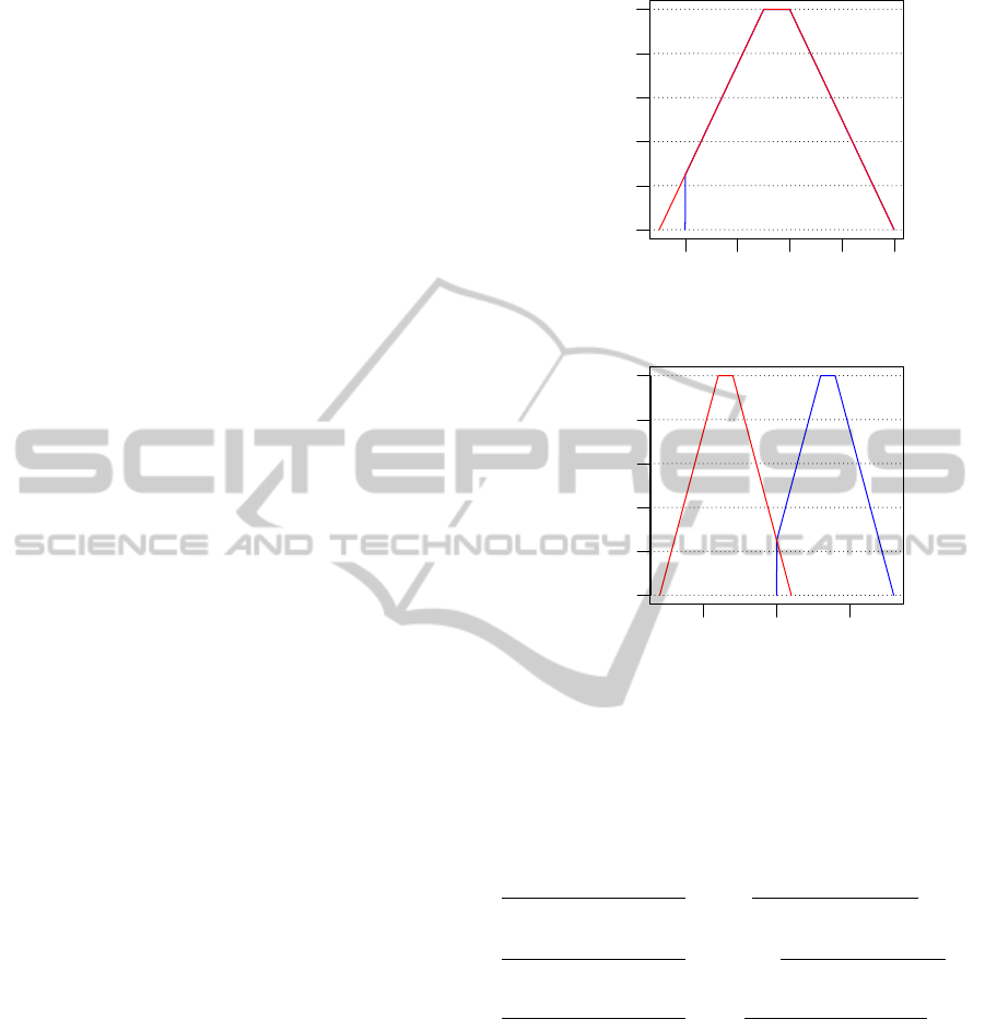
For example, if A
e
= (3, 5, 6, 9) and B
e
=
(1, 2, 2, 4) we can see in Figure 1 that by using (13)
in (12), the negative side of the TrFN is truncated and
the distance between two TrFN is not a TrFN. We will
now prove that by this truncation the GMIR of the dis-
tance between two TrFN’s is bigger than the absolute
value of the GMIR of their difference.
Proposition 1. By Definition 13,
E
A
e
B
e
≤
E
A
e
B
e
.
Proof. Let C
e
= (c
1
, c
2
, c
3
, c
4
) = A
e
B
e
. If c
1
≥ 0,
then µ
C
e
(x) = µ
C
e
(x), ∀x and E
C
e
=
E
C
e
. Con-
0 2 4 6 8
0.0 0.4 0.8
X
µ
a) In red A
e
B
e
and in blue
|
A
e
B
e
|
.
−5 0 5
0.0 0.4 0.8
X
µ
b) In red B
e
A
e
and in blue
|
B
e
A
e
|
.
Figure 1: Manhattan distance between two TrFN.
versely, if c
4
≤ 0, then µ
C
e
(x) = µ
C
e
(−x), ∀x. Thus:
E
C
e
=
E
C
e
−c
4
− 2c
3
− 2c
2
− c
1
6
=
c
1
+ 2c
2
+ 2c
3
+ c
4
6
−c
4
− 2c
3
− 2c
2
− c
1
6
= −
c
1
+ 2c
2
+ 2c
3
+ c
4
6
−c
4
− 2c
3
− 2c
2
− c
1
6
=
−c
1
− 2c
2
− 2c
3
− c
4
6
Now, if either c
1
< 0 and c
i
> 0, ∀i ∈ {2, 3, 4}, or
c
i
< 0, ∀i ∈ {1, 2, 3} and c
4
> 0, then the shape of
C
e
is that of the blue fuzzy number in Figure 1.b. With-
out losing any generality let us assume in this part of
the proof that we only have the first case, i.e., c
1
< 0
and c
i
> 0, ∀i ∈ {2, 3,4}. Let us denote by L
C
e
(x), re-
spectively R
C
e
(x), the membership function that de-
fines
C
e
in [0, c
2
], respectively in [c
3
, c
4
]. Then:
ON THE ABSOLUTE VALUE OF TRAPEZOIDAL FUZZY NUMBERS AND THE MANHATTAN DISTANCE OF
FUZZY VECTORS
401

L
C
e
(x) =
x − c
1
c
2
− c
1
(14)
R
C
e
(x) = 1 −
x − c
3
c
4
− c
3
. (15)
Let µ
12
= µ
C
e
(0). By (15):
µ
12
= −
c
1
c
2
− c
1
. (16)
Using (16) as breaking point, we will find E
C
e
:
E
C
e
=
R
1
0
µ
2
L
−1
C
e
(µ) + R
−1
C
e
(µ)
!
dµ
R
1
0
µdµ
=
R
µ
12
0
µ
2
L
−1
C
e
(µ) + R
−1
C
e
(µ)
!
dµ
R
1
0
µdµ
+
R
1
µ
12
µ
2
L
−1
C
e
(µ) + R
−1
C
e
(µ)
!
dµ
R
1
0
µdµ
By (13) , L
−1
C
e
(µ) = 0, µ ∈ [0, µ
12
]. Thus:
E
C
e
=
R
µ
12
0
µ
2
R
−1
C
e
(µ)
!
dµ
R
1
0
µdµ
+
R
1
µ
12
µ
2
L
−1
C
e
(µ) + R
−1
C
e
(µ)
!
R
1
0
µdµ
dµ
=
c
1
+ 2c
2
+ 2c
3
+ c
4
6
−
c
1
3
6(c
1
− c
2
)
2
.
Now, we state the proposition:
E
C
e
≤ E
C
e
c
1
+2c
2
+2c
3
+c
4
6
≤
c
1
+2c
2
+2c
3
+c
4
6
−
c
1
3
6
(
c
1
−c
2
)
2
c
1
3
(c
1
− c
2
)
2
≤ 0. (17)
The denominator of (17) is always positive, while
the numerator is always negative, thus, proving the
proposition. In the final case, c
1
≤ c
2
< 0 and 0 <
c
3
≤ c
4
. If E(C
e
) > 0 then
C
e
= (0, 0, c
3
, c
4
), else
C
e
= (0, 0, −c
2
, −c
1
). Again, without any lack of
generality, we will prove the proposition for the first
case only:
E
C
e
=
R
1
0
µ
2
L
−1
C
e
(µ) + R
−1
C
e
(µ)
!
dµ
R
1
0
µdµ
.
For this case L
−1
C
e
(µ) = 0, µ ∈ [0, 1], thus:
E
C
e
=
R
1
0
µ
2
R
−1
C
e
(µ)
!
dµ
R
1
0
µdµ
=
2c
3
+ c
4
6
.
Stating the proposition:
E
C
e
≤ E
C
e
c
1
+ 2c
2
+ 2c
3
+ c
4
6
≤
2c
3
+ c
4
6
c
1
+ 2c
2
6
≤ 0. (18)
As both c
1
and c
2
are negative, the proposition is
proved.
So, not only using Dubois and Prade’s definition
makes that the absolute value of a TrFN is not always
a TrFN, but it also overestimates the expected value
obtained by (8). There is a third problem that we will
see now.
Proposition 2. By Definition 13, E
A
e
A
e
6= 0.
Proof. By Definition 11:
A
e
A
e
= A
e
⊕A
e
−
= (a
1
− a
4
, a
2
− a
3
, a
3
− a
2
, a
4
− a
1
) ,
which is a symmetric, zero centered TrFN. By Defini-
tion 13, the absolute value of a symmetric, zero cen-
tered TrFN is a TrFN that only covers the right side
of the first one, i.e.,
A
e
A
e
= (0, 0, a
3
− a
2
, a
4
− a
1
),
thus E
A
e
A
e
6= 0.
A second definition of the absolute value of a
TrFN is directly based on the GMIR, defuzzifying the
fuzzy number to determine whether it is positive or
not.
Definition 14. Given a TrFN M
e
, by means of (8):
M
e
< 0, if E(M
e
) < 0,
M
e
= 0, if E(M
e
) = 0,
M
e
> 0, if E(M
e
) > 0.
Definition 15 ((Chen and Wang, 2008)). The abso-
lute value of a TrFN M
e
is:
M
e
=
M
e
, if M
e
> 0,
0, if M
e
= 0,
M
e
−
, if M
e
< 0.
(19)
FCTA 2011 - International Conference on Fuzzy Computation Theory and Applications
402

This definition of the absolute value has two ad-
vantages over that of (Dubois and Prade, 1979). In
first place,
A
e
B
e
is always a TrFN, and in second
place, E
A
e
A
e
= 0, as A
e
A
e
is a symmetric, zero
centered TrFN.
Nonetheless, it has a problem of its own. As there
is no transformation in shape, the absolute value of a
TrFN might have negative values. For example, if C
e
=
(−1, 2, 4, 6), then E
C
e
=
−1+2·2+2·4+6
6
= 2.833 > 0,
so
C
e
= C
e
= (−1, 2, 4, 6). This result is particularly
problematic for a distance, that by definition cannot
be negative.
There is a second problem with the definition of
(Chen and Wang, 2008) when we use it for the Man-
hattan distance. As the distance goes to zero, so must
do it the uncertainty that about it we have, which is
modeled by the area covered by the TrFN. In mathe-
matical terms, this means that:
lim
E
d
H
e
A
e
,B
e
→0
Z
d
H
f
A
e
, B
e
dx = 0. (20)
In the following proposition, we will see this is
not the behavior of the Manhattan distance based on
Definition 15.
Proposition 3. By Definitions 12 and 15, ∃A
e
, B
e
:
lim
E
d
H
e
A
e
,B
e
→0
R
d
H
f
A
e
, B
e
dx 6= 0.
Proof. From (12) and (19):
d
H
f
A
e
, B
e
= 0 ⇐⇒ E
d
H
f
A
e
, B
e
= 0
E
d
H
f
A
e
, B
e
= 0 ⇐⇒ E
A
e
B
e
= 0 .
Let’s define the zero centered, symmetric TrFN
C
e
= A
e
B
e
= (c
1
, c
2
, c
3
, c
4
) = (−c
4
, −c
3
, c
3
, c
4
) , that
is:
−c
4
= a
1
− b
4
= −a
4
+ b
1
−c
3
= a
2
− b
3
= −a
3
+ b
2
c
3
= a
3
− b
2
c
4
= a
4
− b
1
.
Now, by (8):
E
C
e
=
c
1
+ 2 · c
2
+ 2 · c
3
+ c
4
6
=
−c
4
− 2 · c
3
+ 2 · c
3
+ 2 · c
4
6
= 0,
thus
C
e
= 0 and
R
C
e
dx = 0. Now, if a scalar ε is
added to A
e
, then:
A
0
e
= A
e
+ ε = (a
1
+ ε, a
2
+ ε, a
3
+ ε, a
4
+ ε) ,
so C
0
e
= A
0
e
B
e
= (c
0
1
, c
0
2
, c
0
3
, c
0
4
) and:
c
0
1
= a
0
1
− b
0
4
= a
1
− b
4
+ ε = c
1
+ ε
c
0
2
= a
0
2
− b
0
3
= a
2
− b
3
+ ε = c
2
+ ε
c
0
3
= a
0
3
− b
0
2
= a
3
− b
2
+ ε = c
3
+ ε
c
0
4
= a
0
4
− b
0
1
= a
4
− b
1
+ ε = c
4
+ ε.
Then:
E
C
0
e
=
c
0
1
+ 2 · c
0
2
+ 2 · c
0
3
+ c
0
4
6
=
1
6
((−a
4
+ b
1
+ ε) + 2 (−a
3
+ b
2
+ ε)+
2(a
3
− b
2
+ ε) + (a
4
− b
1
+ ε))
= ε
thus, ∀ε 6= 0,
C
0
e
6= 0 and:
Z
C
0
e
dx =
1
2
−c
0
1
+ c
0
4
=
1
2
(−c
1
− ε + c
4
+ ε)
=
1
2
(c
4
+ c
4
)
= c
4
6= 0.
So, when ε = 0,
R
C
0
e
= 0, but when ε 6= 0,
R
C
0
e
= c
4
. Now, let us suppose c
4
finite but arbitrary
big and ε 6= 0 but infinitesimally small; thus, uncer-
tainty on the distance is very big, even if its expected
value is almost zero. To further observe this behavior,
we calculated d
H
f
A
e
, B
e
, ∀A
e
= (a
1
, a
2
, a
3
, a
4
), B
e
=
(b
1
, b
2
, b
3
, b
4
) : a
i
, b
i
∈ {0, 0.1, . . . , 1}, i = 1, . . . , 4. In
Figure 2 we can see how entropy evolves when ex-
pected distance goes to zero, showing in a black line
the average entropy, in blue its the first and third quar-
tiles, and in red the minimum and maximum entropy
1
.
Except for the case of the minimum , the remaining
curves show what we have already proved in Proposi-
tion 3, i.e., entropy does not go to zero when expected
distance does so; but not only this, it grows, and only
becomes zero for the particular case of P
A
e
, B
e
= 0.
4 MANHATTAN DISTANCE WITH
POSITIVE CORRECTION
The main goal is, therefore, to have a new definition
of the absolute value that takes the positive aspects
1
Irregularities in Figure 2 come from the discrete way
in which fuzzy numbers were generated. This behavior
should disappear by increasing granularity, but in turn, this
increases computational complexity.
ON THE ABSOLUTE VALUE OF TRAPEZOIDAL FUZZY NUMBERS AND THE MANHATTAN DISTANCE OF
FUZZY VECTORS
403

0.0 0.2 0.4 0.6 0.8 1.0
0.0 0.5 1.0 1.5 2.0
((d ((A,, B ))))
⌠⌠
⌡⌡
d ((A,, B ))d x
E
Figure 2: Entropy of the Manhattan distance as a function
of its GMIR, in the interval [0,1].
of both, Definitions 13 and 15, i.e., that the absolute
value of a TrFN removes negative values, keeping the
same expected value of the TrFN obtained through
(8). For this, we will define what we have termed as
“positive correction”.
Definition 16. The “positive correction”
7→
A
e
of a TrFN
A
e
= (a
1
, a
2
, a
3
, a
4
) is defined as:
7→
A
e
=
(a
1
,a
2
,a
3
,a
4
), if a
1
≥0,
(0,a
2
−γ
1
,a
3
−γ
1
,a
4
−γ
1
), if a
1
<0 and
a
1
5
+a
2
≥0,
(0,0,a
3
−γ
2
,a
4
−γ
2
), if a
2
+
a
1
5
<0
and
a
1
3
+
2a
2
3
+a
3
≥0,
(0,0,0,a
4
−γ
3
), if
a
1
3
+
2a
2
3
+a
3
<0,
(0,0,0,0), else.
(21)
Proposition 4. For a TrFN A
e
= (a
1
, a
2
, a
3
, a
4
), such
that a
1
< 0 and a
2
+
a
1
5
≥ 0, then:
γ
1
= −
a
1
5
.
Proof. Let us recall the two conditions that the posi-
tive correction of a TrFN should meet: (i) there should
be no negative values, i.e.,
7→
a
1
= 0, and (ii) the ex-
pected value according to (8) must be kept the same.
To comply with both conditions we must establish the
following equality:
E
A
e
= E
7→
A
e
a
1
+2a
2
+2a
3
+a
4
6
=
2
(
a
2
−γ
1
)
+2
(
a
3
−γ
1
)
+
(
a
4
−γ
1
)
6
a
1
6
= −
5 · γ
1
6
γ
1
= −
a
1
5
.
Due to the first condition and by definition of
TrFN a
2
− γ
1
≥ 0, then a
2
+
a
1
5
≥ 0.
Proposition 5. For a TrFN A
e
= (a
1
, a
2
, a
3
, a
4
), such
that a
2
+
a
1
5
< 0 and
a
1
3
+
2·a
2
3
+ a
3
≥ 0, then:
γ
2
= −
a
1
3
−
2 · a
2
3
.
Proof. Again, we state the equality:
E
A
e
= E
7→
A
e
,
but this time
7→
a
1
=
7→
a
2
= 0 for
7→
A
e
, thus:
a
1
+ 2a
2
+ 2a
3
+ a
4
6
=
2(a
3
− γ
2
) + (a
4
− γ
2
)
6
a
1
+ 2a
2
6
= −
γ
2
2
γ
2
= −
a
1
3
−
2a
2
3
.
Due to the first condition of the positive correction
and by definition of TrFN a
3
−γ
2
≥ 0, then
a
1
3
+
2a
2
3
+
a
3
≥ 0.
Proposition 6. For a TrFN A
e
= (a
1
, a
2
, a
3
, a
4
), such
that
a
1
3
+
2a
2
3
+ a
3
< 0 then:
γ
3
= −x
1
− 2x
2
− 2x
3
.
Proof. One last time, we state the equality:
E
A
e
= E
7→
A
e
,
only this time
7→
a
1
=
7→
a
2
=
7→
a
3
= 0 for
7→
A
e
, thus:
a
1
+ 2a
2
+ 2a
3
+ a
4
6
=
(a
4
− γ
3
)
6
a
1
+ 2a
2
+ 2a
3
6
= −
γ
3
6
γ
3
= −a
1
− 2a
2
− 2a
3
.
Due to the first condition of the positive correction
and by definition of TrFN a
4
−γ
3
≥ 0, then a
1
+2a
2
+
2a
3
+ a
4
≥ 0.
Once defined the positive correction of a TrFN,
we present the new absolute value of a TrFN as well
as the Manhattan distance for two TrFNs.
Definition 17. The absolute value of a TrFN A
e
is de-
fined as:
A
e
=
7→
A
e
, if E (A
e
) > 0,
0, if E (A
e
) = 0,
7→
A
e
−
, if E (A
e
) < 0.
(22)
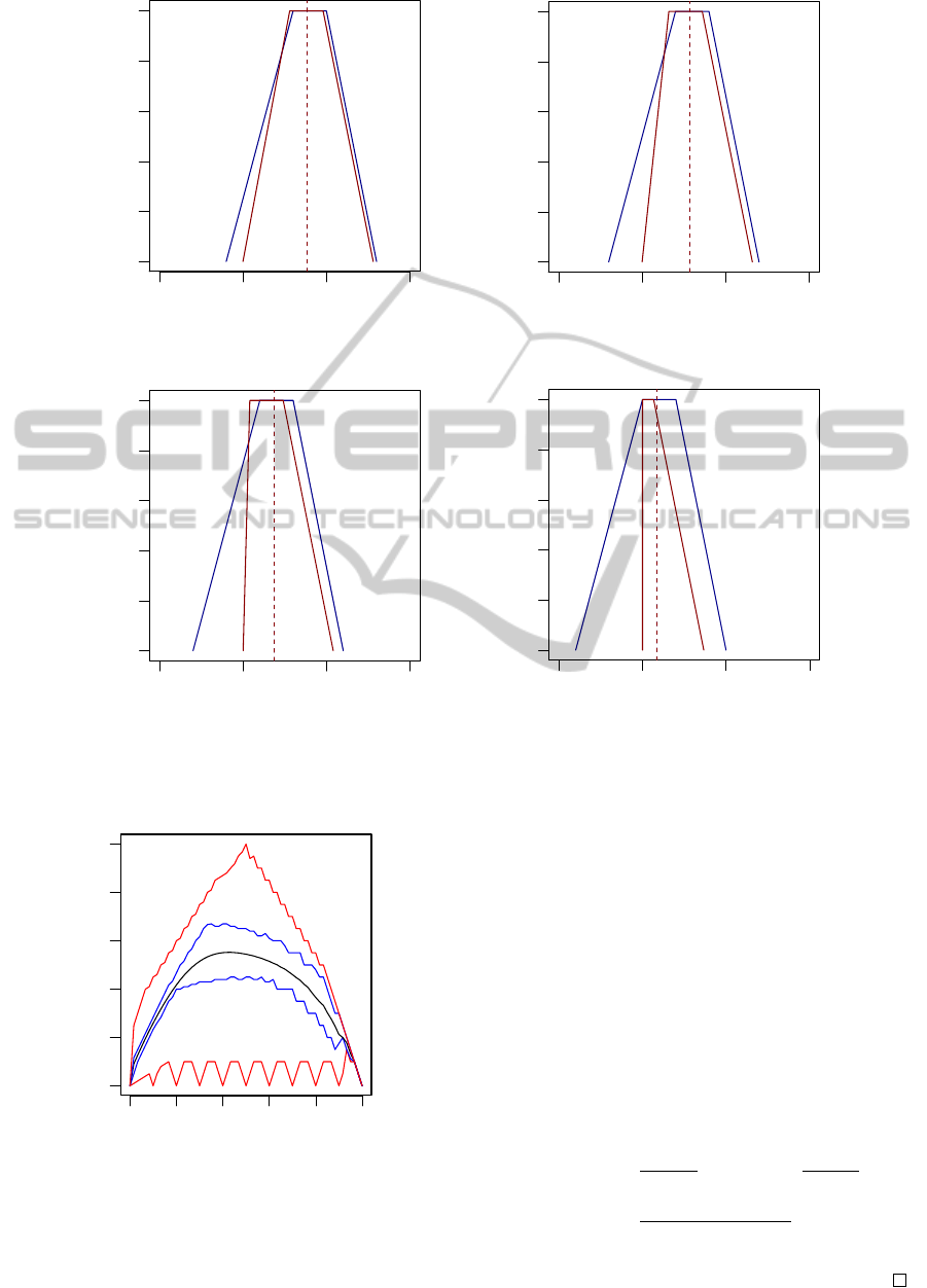
Figure 3 shows that by using the positive correc-
tion in the absolute value, the uncertainty of the Man-
hattan distance goes to a maximum, top red line, when
the GMIR is close to 0.5.
FCTA 2011 - International Conference on Fuzzy Computation Theory and Applications
404
−0.5 0.0 0.5 1.0
0.0 0.2 0.4 0.6 0.8 1.0
X
µ
−0.5 0.0 0.5 1.0
0.0 0.2 0.4 0.6 0.8 1.0
X
µ
a) d (A
e
, B
e
) b) d (A
e
− .1, B
e
)
−0.5 0.0 0.5 1.0
0.0 0.2 0.4 0.6 0.8 1.0
X
µ
−0.5 0.0 0.5 1.0
0.0 0.2 0.4 0.6 0.8 1.0
X
µ
c) d (A
e
− .2, B
e
) d) d (A
e
− .3, B
e
)
Figure 4: Manhattan distance calculated with the absolute value of Chen and Wang (in blue) and with the positive correction
(in red), as well as the expected value calculated through the GMIR (dashed red line).
0.0 0.2 0.4 0.6 0.8 1.0
0.0 0.2 0.4 0.6 0.8 1.0
((d ((A,, B ))))
E
⌠⌠
⌡⌡
d ((A,, B ))d x
Figure 3: Entropy of the Manhattan distance with positive
correction as a function of its GMIR, in the interval [0,1].
Proposition 7. For any two TrFN A
e
=
(a
1
, a
2
, a
3
, a
4
), B
e
= (b
1
, b
2
, b
3
, b
4
) such that a
1
≥ 0,
b
1
≥ 0, a
4
≤ 1, b
4
≤ 1, and E
A
e
≥ E
B
e
,
argmax
d
H
e
A
e
,B
e
Z
1
0
d
H
f
A
e
, B
e
dx = (0, 0, 1, 1) .
Proof. Given that for any two TrFN A
e
and B
e
, as de-
fined by the proposition, by Definitions 16 and 17
d
H
f
A
e
, B
e
is always a TrFN such that C
e
= d
H
f
A
e
, B
e
=
(c
1
, c
2
, c
3
, c
4
) with c
1
≥ 0 and c
4
≤ 1, then:
max
Z
1
0
C
e
(x) dx
= 1 .
For a TrFN, this integral yields:
Z
1
0
C
e
dx =
c
2
− c
1
2
+ c
3
− c
2
+
c
4
− c
3
2
=
−c
1
− c
2
+ c
3
+ c
4
2
. (23)
It is straightforward to see that (23) maximizes for
C
e
= (0, 0, 1, 1), and that E
C
e
= 0.5.
ON THE ABSOLUTE VALUE OF TRAPEZOIDAL FUZZY NUMBERS AND THE MANHATTAN DISTANCE OF
FUZZY VECTORS
405

We can also see in Figure 3, that the main objec-
tive pursued, i.e., that uncertainty goes to zero with
the expected value of the distance, is achieved with
the positive correction of the Manhattan distance. In
Figure 4 we can see an example calculating d
H
f
A
e
, B
e
for A
e
= (.3, .6, .7, .9) and B
e
= (.1, .2, .3, .4), using
Chen and Wang’s absolute value (in blue) and the pos-
itive correction (in red). We can see how the positive
correction removes the negatives values of d
H
f
A
e
, B
e
,
but maintains its GMIR (dashed red line), accom-
plishing the second objective originally proposed.
5 CONCLUSIONS
In this paper, we have discussed on the definition of
the absolute value of a TrFN and its role on the cal-
culation of the Manhattan distance for fuzzy vectors.
The first definition studied, the one made by (Dubois
and Prade, 1979), has two problems. Firstly, the re-
sulting distance might not be a TrFN, which compli-
cates following calculations. Secondly, depending on
the the TrFN, it might overestimate the absolute value
of its GMIR or expected value.
The second definition evaluated, that of (Chen and
Wang, 2008), solves these problems but introduces
some problems of its own. Firstly, the absolute value
of a TrFN might have has negative values, which goes
against all sense when modeling distances and their
uncertainty. Secondly, it violates another common-
sense condition of distances: its uncertainty must go
to zero when the distance does too.
To solve these new problems we present a method
called “positive correction”, in which we remove neg-
ative values while keeping the same expected value,
leaving the distance as a TrFN. The result is a distance
that captures uncertainty, but that also stays close to
the conception that distances have in the real world.
REFERENCES
Chen, S.-H. and Hsieh, C.-H. (1999). Graded mean integra-
tion representation of generalized fuzzy number. Jour-
nal of Chinese Fuzzy System, 5(2):1–7.
Chen, S.-H. and Wang, C.-C. (2008). Fuzzy distance of
trapezoidal fuzzy numbers and application. Interna-
tional Journal of Innovative Computing, Information
and Control, 4(6):2008.
Dubois, D. and Prade, H. (1979). Fuzzy real algebra: some
results. Fuzzy Sets and Systems, 2:327–348.
Kaufmann, A. and Gupta, M. M. (1985). Introduction to
Fuzzy Arithmetic. Van Nostrand Reinhold, New York.
Li, X. and Liu, B. (2008). On distance between fuzzy
variables. Journal of Intelligent and Fuzzy Systems,
19:197–204.
Tran, L. and Duckstein, L. (2002). Comparison of fuzzy
numbers using a fuzzy distance measure. Fuzzy Sets
and Systems, 130:331–341.
Voxman, W. (1998). Some remarks on distances between
fuzzy numbers. Fuzzy Sets and Systems, 100:353–
365.
Zadeh, L. (1965). Fuzzy sets. Information and Control,
8(3):338–353.
Zadeh, L. (1975). The concept of a linguistic variable and
its application to approximate reasoning - i. Informa-
tion Sciences, 8:199–249.
Zimmermann, H.-J. (2005). Fuzzy Sets: Theory and its Ap-
plications. Springer, 4 edition.
FCTA 2011 - International Conference on Fuzzy Computation Theory and Applications
406
