IMPROVING THE PERFORMANCE OF THE SUPPORT

VECTOR MACHINE IN INSURANCE RISK CLASSIFICATION

A Comparitive Study

Mlungisi Duma, Bhekisipho Twala, Tshilidzi Marwala

Department of Electrical Engineering and the Built Environment, University of Johannesburg APK

Corner Kingsway and University Road, Auckland Park, Johannesburg, South Africa

Fulufhelo V. Nelwamondo

Council for Scientific and Industrial Research (CSIR), Pretoria, South Africa

Keywords: Support vector machine, Principal component analysis, Genetic algorithms, Artificial neural network,

Autoassociative network, Missing data.

Abstract: The support vector machine is a classification technique used in linear and non- linear complex problems. It

was shown that the performance of the technique decreases significantly in the presence of escalating

missing data in the insurance domain. Furthermore the resilience of the technique when the quality of the

data deteriorates is weak. When dealing with missing data, the support vector machine uses the mean-mode

strategy to replace missing values. In this paper, we propose the use of the autoassociative network and the

genetic algorithm as alternative strategies to help improve the classification performance as well as increase

the resilience of the technique. A comparative study is conducted to see which of the techniques helps the

support vector machine improve in performance and sustain resilience. The training data with completely

observable data is used to construct the support vector machine and testing data with missing values is used

to measuring the accuracy. The results show that both models help increase resilience with the

autoassociative network showing better overall performance improvement.

1 INTRODUCTION

Insurance industries have played a crucial role in

carrying risks on behalf of clients since their

inception in the late seventeenth century. These risks

include carrying the cost of a patient admitted to a

hospital, vehicle repairs for a client involved in a car

accident and many other incidents. However,

numerous people today still do not have an

insurance cover. The first well-known reason is

refusing to get a cover (Crump, 2009); (Howe,

2010). Many people believe that insurance

companies are there to make profits rather than

helping their clients. Therefore they would rather

save their money and incur the risk of paying the

cost if any catastrophic event happens to them

(Crump, 2009). The second common reason is

cancellation. Fraud, failing to pay premiums on time

or numerous claims results in client policies being

terminated by the insurer (Crump, 2009); (Howe,

2010). The third common reason is affordability

(Howe, 2010). The premiums for a cover may be

very expensive due to increasing premiums. A client

is therefore forced to cancel the cover.

In this paper, a solution to improve the support

vector machine (SVM) as a predictive modelling

technique in the insurance risk classification is

presented. The solution improves the manner in

which client risk is predicted using new data. The

model is trained using past data (with a large number

of features) about clients who are likely to have

insurance cover. This information is then used to

predict the future behaviour of a new client. The

new client data in this case, has attributes with

missing values. Missing values are due to clients

failing to supply the data, or processing error by the

system handling the data (Duma et al., 2010).

Support vector machines struggle with

classification performance compared to other

supervised algorithms (such as the naïve Bayes, k-

340

Duma M., Twala B., Marwala T. and V. Nelwamondo F..

IMPROVING THE PERFORMANCE OF THE SUPPORT VECTOR MACHINE IN INSURANCE RISK CLASSIFICATION - A Comparitive Study.

DOI: 10.5220/0003673803400346

In Proceedings of the International Conference on Neural Computation Theory and Applications (NCTA-2011), pages 340-346

ISBN: 978-989-8425-84-3

 2011 SCITEPRESS (Science and Technology Publications, Lda.)

Nearest Neighbour, and the logical discriminant

algorithms) if new data contains missing data (Duma

et al., 2010). One of the main reasons is over-fitting

of the data. Even though support vector machines

are designed to be less prone to over-fitting, in very

high dimensional space, this problem cannot be

avoided. When training support vector machines, a

lot of detail is learned if the client data has many

attributes. The result of this is incorrect predictions

of new client data, especially if new data is of poor

quality as a result of missing values. The model also

has little resilience in the presence of increasing

missing data. In comparison with other supervised

learning models, its classification performance

decreased sharply when the quality of the data

deteriorated.

We present a comparative study on genetic

algorithms and autoassociative networks as effective

models to help improve the classification of the

support vector machines and increase resilience.

Genetic algorithms have been applied successfully

as methods for optimising classification algorithms,

(Chen et al., 2008); (Minaei-Bidgoli et al., 2004). It

has also been applied in fault classification of

mechanical systems as a method for estimating

missing values (Marwala et al., 2006).The

autoassociative networks have been applied

successfully in HIV classification (Leke et al.,

2006), missing data imputation (Marivate et al.,

2007) and assisting in image recognition (Pandit et

al., 2011).

We also employ the use of the principal

component analysis (PCA) as a feature selection

technique to reduce over-fitting and computational

cost. Principal component analysis removes those

dimensions that are not relevant for classification.

The reduced dataset in then passed on to the support

vector machine to learn. Principal component

analysis has been applied successfully in fault

identification and analysis of vibration data

(Marwala, 2001). Is has also been used in automatic

classification of ultra-sound liver images

(Balasubramanian et al., 2007) and in identifying

cancer molecular patterns in micro-array data (Han,

2010).

The rest of the paper is organised as follows:

Section 2 gives a background discussion on the

support vector machine, the principal component

analysis, genetic algorithms, autoassociative

networks and missing data mechanisms. Section 3 is

a discussion on the datasets and pre-processing. A

discussion on the AN-SVM structure and the GA-

SVM structure is also given. Section 4 is a

discussion on the experimental results. Conclusion

and future works is discussed in section 5.

2 BACKGROUND

2.1 Support Vector Machine

Support vector machine is a classification method

applied to both linear and non-linear complex

problems (Steeb, 2008). It makes use of a non-linear

mapping to transform data from lower to higher

dimensions. In the higher dimension, it searches for

an optimal hyper-plane that separates the attributes

of one class to another. If the data set is linearly

separable (i.e. a straight line can be drawn to

separate all attributes of a one class from all

attributes of another), the support vector machine

finds the maximal marginal hyper-plane, i.e. the

hyper-plane with the greatest margin. The separation

satisfies the following equation (Steeb, 2008),

(1)

where  is the weight vector and  is the input

vector. A larger margin allows classification of new

data to be more accurate. If the data set is linearly

inseparable, the original data is transformed into a

new higher dimension. In the new dimension, the

support vector machine searches for an optimal

hyper-plane that separates the attributes of the

classes. The maximal marginal hyper-plane found in

the new dimension corresponds to the non-linear

surface in the original space. The mapping of input

data into higher dimensions is performed by kernel

functions expressed in the form (Steeb, 2008),

(2)

where and are nonlinear mapping

functions. There are three commonly used kernel

functions used to training attributes into higher

dimensions, namely the polynomial, Gaussian radial

basis and sigmoid function (Steeb, 2008). In this

paper, we use the Gaussian radial basis function.

Support vector machines have been applied

successfully in the insurance industry

and in credit

risk analysis. They have been used to help identify

and manage credit risk (Chen et al, 2009, Yang et al,

2008). They have also been employed to predict

insolvency (Yang et al, 2008).

2.2 Principal Component Analysis

Principal component analysis (PCA) is a popular

IMPROVING THE PERFORMANCE OF THE SUPPORT VECTOR MACHINE IN INSURANCE RISK

CLASSIFICATION - A Comparitive Study

341

feature extraction technique used to find patterns in

data with many attributes and reduce the number of

attributes (Marwala, 2009).

In most instances, the goal of the principal

component analysis is to compress the dimensions of

the data whilst preserving as much as possible the

representation of the original data. The first step is

determining the average of each dimension and then

subtract from the values of the data. The covariance

matrix of the data set is then calculated. The eigen-

values and the eigen-vectors are determined using

the covariance matrix as a basis. At this point, any

vector dimension or its average can be expressed as

a linear combination of the eigenvectors. The last

step is choosing the highest eigen-values that

correspond to the largest eigenvectors, or the

principal components. The last step is where the

concept of data compression comes into effect. The

eigen-values that are chosen along with their

corresponding eigenvectors are used to reduce the

number of dimensions whilst preserving most

information (Marwala, 2009). This reduction can be

expressed as

[P] = [M] x [N] (3)

where [P] represents the transformed data set, [M]

represent the given data set and [N] is the principal

component matrix. [P] represents a dataset that

expresses the relationships between the data

regardless of whether the data has equal or lower

dimension. The original data set can be calculated

using the following equation

[M’] = [P] x [N

-1

] (4)

where [M’] represents the re-transformed data set

and [M’] ≈ [M] if all the data from [N

-1

] is used from

the covariance matrix.

2.3 Genetic Algorithm

Genetic algorithm (GA) is an evolutionary

computational model that is used to find global

solutions to complex problems (Michalewicz, 1996).

Genetic algorithms are inspired by Darwin’s theory

of natural evolution. They use the concept of

survival of the fittest over a number of generations

to find the optimal solution to a problem. In a

population, the fittest individuals are selected for

reproduction. The selection process is based on a

probabilistic technique that ensures that the strongest

individuals are chosen for reproduction. There are

various techniques that can be used for selection,

namely the roulette wheel selection, ranking

selector, tournament selection and stochastic

universal sampling (Michalewicz, 1996). The

roulette wheel selection uses a structure where each

individual has a roulette wheel slot size that is in

proportion to its fitness. The ranking selector orders

individuals according to their probability for

selection. The tournament selection technique

selects a random numbers of individuals, and then

assigns the highest probability to the fittest two

individuals. The stochastic universal sampling

technique is an alternative to the roulette wheel

selection. The technique ensures that the selection of

each individual is regular with its expected rate of

selection. In this paper, we use the roulette wheel

selection as it is a commonly used technique for

selection (Marwala, 2009).

After the selection process, steps involving

crossover, mutation and recombination are

performed to generate new individuals (Marwala,

2007, Steeb, 2008).

Crossover involves selecting a crossover point

between two parent individuals or chromosomes

(This can be a point in a string of bits or an array of

features that represent an instance in a dataset). Data

from the beginning of a chromosome to the

crossover point is exchange with another parent

chromosome. The results are two child

chromosomes. Mutation involves selecting a random

gene to invert it. It usually has a very low probability

of occurring than the crossover process (i.e. less than

1%). Recombination involves evaluating the fitness

value of the new individual to determine if they can

be recombined with the existing population. The

weakest individuals are removed from the

population (Marwala, 2007, Steeb, 2008).

2.4 Autoassociative Network

Autoassociative networks are specialized neural

networks that are designed to recall their inputs. This

implies that the input values supplied to the network

are the predicted output representing the inputs. The

number of hidden inputs in the hidden layer is often

less than the number of inputs. The number of

hidden layers cannot be too small otherwise the

learning results in poor generalisation and prediction

accuracy (Leke et al, 2006). In a classification

problem, the inputs vectors x ∈ℝ



include the

class value. The predicted values y∈  ℝ



are

expressed in the following form

=



(, )

(5)

where arethe mapping weights. The error function

e between the input vectors as well as the predicted

outputs, can be expressed in the form

NCTA 2011 - International Conference on Neural Computation Theory and Applications

342

=−

(6)

By squaring the error function and replaying  with

equation (5) (Leke et al, 2006), we get

=(−



(, ))



(7)

we obtain the minimum and non-negative error,

which is what is required for the work presented in

this paper. Equation (7) can be expressed as a scalar

by integrating over the input vectors an the number

of training examples as follows

E =

‖

−



(, )

‖

(8)

where

‖‖

represents the Euclidean norm. The

minimum error is obtained when the outputs are the

closest matching to the inputs.

2.5 Missing Data Mechanisms

Information that is gathered from various sources

can have missing data. There are various reasons for

missing data. Some include people refusing to

disclose certain information for privacy or security

reasons, faulty processing by system and systems

exchanging information that has missing data

(Francis, 2005).

The mechanisms for handling missing data are

missing at random, missing completely at random,

missing not at random and missing by natural design

(Little et al, 1987, Marwala, 2009). Missing

complete at random infers that the missing data is

independent of any other existing data. Missing at

random infers that the missing data is not related to

the missing variables themselves but to other

variables. Missing not at random infers that the

missing data depends on itself and not on any other

variables. Missing by natural design infers that the

data is missing because the variable is naturally

deemed un-measurable, even though they are useful

for data analysis. Therefore, the missing values are

modelled using mathematical techniques (Marwala,

2009).

In this paper, we infer that the data is missing

completely at random. The reason is that single and

multiple imputations return unbiased estimates.

3 METHODS

3.1 Datasets and Pre-processing

There are two datasets used for conducting the

experiment. Both dataset are executed separately and

their results are combined. The first dataset is the

Texas insurance dataset used by the Texas

government to draw up the Texas Liability Insurance

Closed Claims Report. The report contains a

summary of medical insurance claims for various

injuries. The claims are either short form or long

form. Short form claims are associated with small

injuries that are not expensive for individuals to pay

for themselves. Long-term form claims are

associated with major injuries that are expensive and

require medical insurance. In this dataset, we

classify instances based on whether they have

medical insurance cover for long form claims as a

risk analysis exercise, provided there is missing

information.

The Texas Insurance dataset has over 9000

instances, which were reduced manually to 5446

instances by removing all the short form claims. The

dataset is separated into training and testing datasets,

1000 and 500 instances respectively (the datasets

were reduced to help increase the speed of the

training and testing processes. The instances were

also randomly chosen). Both sets have missing

values initially. We use the testing set to simulate

missing data. Each set consists of a total of over 220

attributes initially. The attributes were reduced

manually to 118 attributes by manually removing

those attributes that were not significant for the

experiment such as unique identities, dates etc. The

data was also processed to have categorical

numerical values for each attribute. The class

attribute used also has two values (0 to indicate no

medical insurance and 1 to indicate that the claimer

has medical insurance).

The second insurance dataset is from the

University of California Irvine (UCI) machine

learning repository. The dataset is used to predict

which customers are likely to have an interest in

buying a caravan insurance policy. In this paper, we

use it to find out customers who are likely to have a

car insurance policy for their motor vehicles,

provided there is missing data in the information

The training dataset has over 5400 instances of

which 1000 were used for the experiment. The

testing dataset consists of only 4000 instances of

which 800 instances were randomly chosen and

used. Analogous to the Texas Insurance dataset, the

subsets of the UCI training and testing datasets are

used so that the experiment runs at optimum speed.

Each set has a total of 86 attributes with completely

observable data, 5 of which are categorical numeric

values and 80 are continuous numeric values.

Processing was done to make the data consist of

categorical numeric values. The class attribute

consists of only two values (0 to indicate a customer

IMPROVING THE PERFORMANCE OF THE SUPPORT VECTOR MACHINE IN INSURANCE RISK

CLASSIFICATION - A Comparitive Study

343

that is likely not to have insurance or 1 to indicate a

customer that is likely to have an insurance cover).

There are five levels of proportions of

missingness on the testing datasets that are generated

(10%, 25%, 30%, 40% and 50% respectively). At

each level, the missingness is arbitrarily generated

across the entire datasets, then on half the attributes

of the sets. Therefore, in total, 30 testing datasets

were created for the experiment.

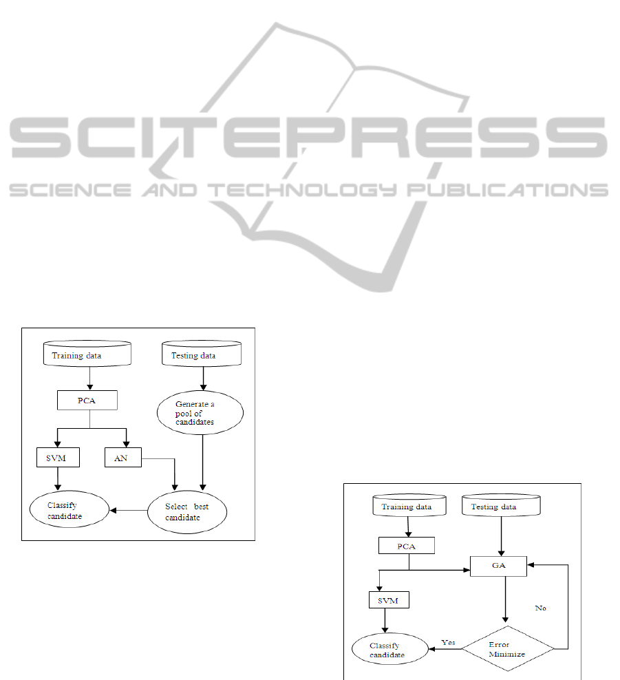
3.2 AN-SVM Structure

Figure 1 shows the structure for improving the

support vector machine using the autoassociative

network. We refer to the structure as the AN-SVM

structure. The initial step is compressing the data

using the principal component technique. The

compressed data is used to construct the

autoassociative network. Once the network is

constructed, it is used to select the best candidate for

the support vector machine to classify. A group of

candidates is created for each instance that has

missing values from the testing data. This is done by

randomly replacing missing entries with values for

each candidate. We create between 10 and 500

candidates for each instance, depending on the

number of missing values. The candidate with the

smallest error according to equation (8) is chosen for

classification. This is done until all instances that

have missing values have a potential candidate.

Figure 1: AN-SVM structure.

The autoassociative network is made up of the

input, hidden and output layers. There are 20 nodes

on hidden layer, determined by trial and error. The

Gaussian function is used as an activation function

between the input and hidden layer. The linear

activation function is used between the hidden and

output layer (Leke et al, 2006). The back-

propagation technique is used for learning and the

number of epochs is 400. The network is written

using C# 3.5 programming language, Weka and

IKVM libraries. The support vector machine is

constructed using Weka 3.6.2 and libSVM 2.91, a

library for tool support vector machines. The radial

basis function was used as the kernel function. The

principal component was also built using the Weka

3.6.2 library.

3.3 GA-SVM Structure

Figure 2 illustrates the genetic algorithm approach to

improving the support vector machine classification

performance. We refer to the structure as the GA-

SVM structure. The initial step is synonymous to the

AN-Structure. The only difference is that the genetic

algorithm is responsible for creating a population of

candidates and selecting the best one for

classification. Each candidate represents a potential

solution, i.e. it can belong to the 0 class or the 1

class. The maximum number of potential candidates

created is 15 for each instance with missing values.

Each candidate is represented as follows:

• Each observable entry is ignored, as illustrated by

the star (*) in figure 3. The other entries contain

generated values used to replace the missing values.

• During the crossover step, only the generated

values are exchanged to generate new individual.

Similarly, mutation step only occurs on entries with

generated values.

Each child candidate’s fitness is evaluated using

equation (8). The roulette wheel selection is used in

the selection step. The genetic algorithm is

constructed using the watch-maker framework 0.7.1.

The number of epochs is 100 and the mutation

probability was 0.0333, as recommended by Leke

(Leke et al, 2006) and Marwala (Marwala et al,

2006).

Figure 2: GA-SVM structure.

NCTA 2011 - International Conference on Neural Computation Theory and Applications

344

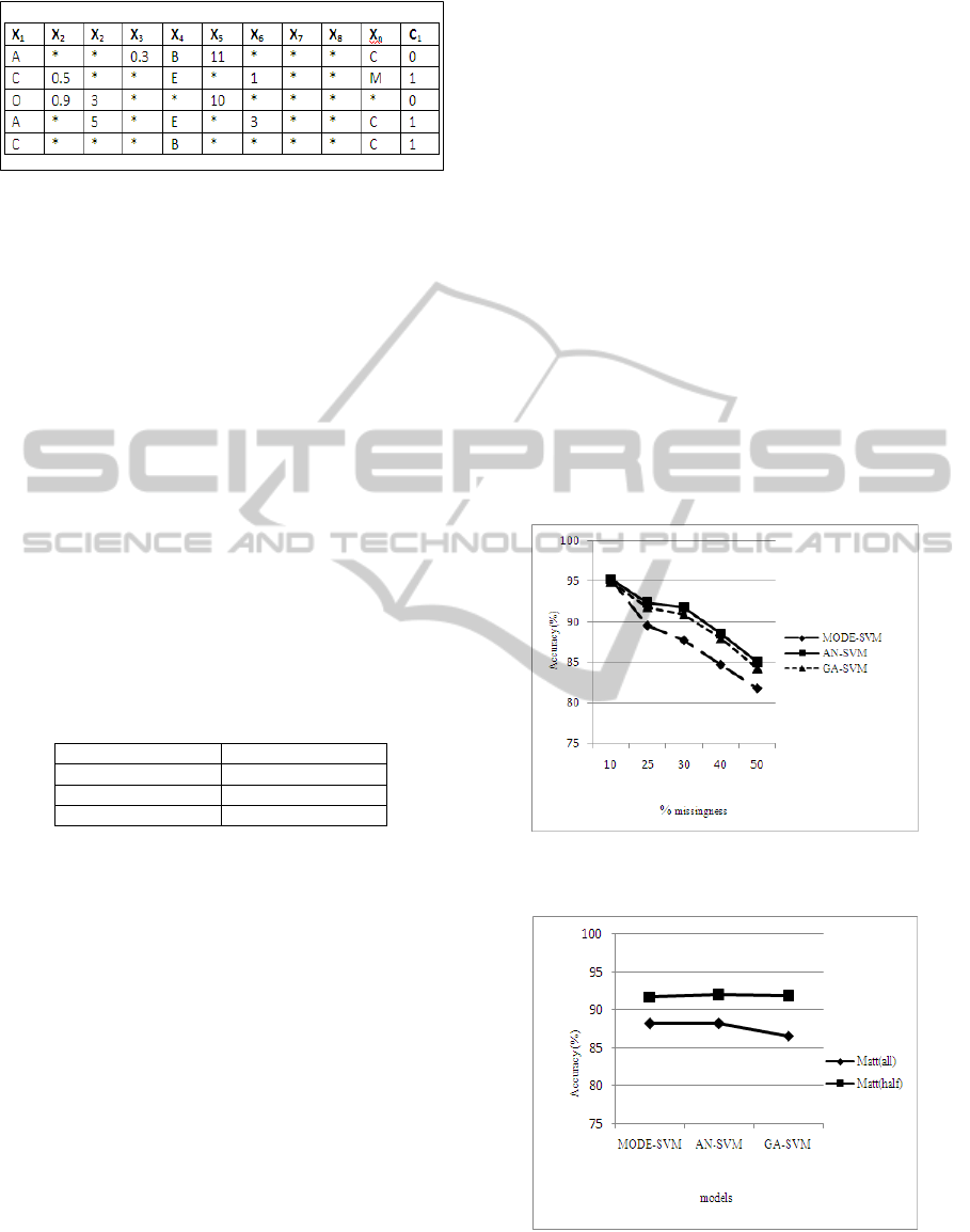
Figure 3: Candidate representation. * means ignored

entries. X

…X

are attributes and C

is the class-label.

4 EXPERIMENT RESULTS

The overall results of the experiment are illustrated

in table 1. The AN-SVM and the GA-SVM are

compared with MODE-SVM, support vector

machine that uses the mean-mode strategy to replace

missing values. All the models perform well overall

with AN-SVM achieving higher accuracies than the

other models by a small margin. The GA-SVM

achieves a lower accuracy than the MODE-SVM.

The reason being is that the MODE-SVM achieves

high accuracies when there is a small percentage of

missing data. Furthermore the GA-SVM struggled

with performance when data was missing across all

attributes compared to other models. This is

illustrated in figure 5.

Table 1: Overall Classification Accuracy.

Accuracy (%)

MODE-SVM 89.94

AN-SVM 90.04

GA-SVM 89.145

The overall performance in figure 4 shows that

the AN-SVM and GA-SVM are more resilient to

escalating missing data than the MODE-SVM. From

figure, the performance of the MODE-SVM

decreases sharply as the quality of the data

deteriorates. The AN-SVM shows more steadiness

in declining performance than the other models.

Figure 6 shows the overall performance of the

models with half or all attributes with missing data.

From the figure, it is clear that all the models

perform well and show more resilience when there is

half the attributes with missing value. In the case

when all or most attributes have missing data, a

sharp decline in performance is experienced when

the percentage of missingness increase above 30%.

The Mode-SVM contributes mostly in the sharp

decrease.

5 CONCLUSIONS AND FUTURE

WORK

We conducted a study using the autoassociative

network and genetic algorithm to help improve the

classification performance of support vector

machines, in the presence of escalating missing data.

Although support vector machines perform well

when using the mean mode technique, the

performance declines sharply when the quality of the

data deteriorates. The autoassociative network

showed better performance than the genetic

algorithm. It also showed better resilience when the

percentage of missing data increased. The genetic

algorithm also showed some resilience.

Future work should focus on improving the

performance of the genetic algorithm by optimizing

the process illustrated in figure 2. The number of

candidates currently chosen is a few and a better

evaluation function can be used.

Figure 4: The overall performance of the MODE-SVM,

AN-SVM and GA-SVM.

Figure 5: Overall performance per model. Matt(all) is

short for most attributes with missing values. Matt(half) is

short for half the attributes with missing values.

IMPROVING THE PERFORMANCE OF THE SUPPORT VECTOR MACHINE IN INSURANCE RISK

CLASSIFICATION - A Comparitive Study

345

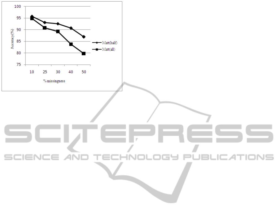
Figure 6: Overall performance with half or all attributes

with missing values. Matt(all) is short for most attributes

with missing values. Matt(half) is short for half the

attributes with missing values.

REFERENCES

Balasubramanian, D., Srinivasan, P., Gurupatham, R.,

2007. Automatic Classification of Focal Lesions in

Ultrasound Liver Images using Principal Component

Analysis and Neural Networks. In AICIE’07, 29th

Annual International Conference of the IEEE EMBS,

pp. 2134 – 2137, Lyon, France.

Bishop, C. M., 1995.Neural Network for Pattern

Recognition. Oxford University Press, New York,

USA.

Chen, M., Zhengwei, Y., 2008. Classification Techniques

of Neural Networks Using Improved Genetic

Algorithms. In ICGEC’08, 2

International

Conference on Genetic and Evolutionary Computing,

pp.115 – 199, IEEE Computer Society, Washington,

DC, USA.

Crump, D., 2009. Why People Don’t Buy Insurance.

Ezine Articles. (Source: http://ezinearticles.com/

?cat=Insurance).

Duma, M., Twala, B., Marwala, T., Nelwamondo, F. V.,

2010. Classification Performance Measure Using

Missing Insurance Data: A Comparison Between

Supervised Learning Models. In ICCCI’10

International Conference on Computer and

Computational Intelligence, pp. 550 - 555, Nanning,

China.

Francis, L., 2005. Dancing With Dirty Data: Methods for

Exploring and Cleaning Data. Casualty Actuarial

Society Forum Casualty Actuarial Society, pp. 198-

254, Virgina, USA. (Source:http://www.casact.org/

pubs/forum/05wforum/05wf198.pdf)

Howe,C., 2010. Top Reasons Auto Insurance Companies

DropPeople.eHow. (Source:http://www.ehow.com/fact

s_6141822_top- insurance-companiesdrop-people.

html).

Leke, B., B., Marwala T., Tettey T., 2006. Autoencoder

Networks for HIV Classification. Current Science,

vol. 91, no. 11.

Little, R., J., A., Rubin, D., B., 1987. Statistical Analysis

with Missing Data. Wiley New York, USA.

Marwala T., 2001. Fault Identification using neural

network and vibration data. Unpublished doctoral

thesis, University of Cambridge, Cambridge.

Marwala, T., Chakraverty, S., 2006. Fault Classification in

Structures with Incomplete Measured Data using

Autoassociative Neural Networks and Genetic

Algorithm. Current Science, vol. 90, no. 4.

Marwala, T., 2007. Bayesian Training of Neural Networks

using Genetic Programming.

Marwala, T., 2009. Computational Intelligence for

Missing Data Imputation Estimation and Management

Knowledge Optimization Techniques, Information

Science Reference, Hershey, New York, USA.

Marivate, V., N., Nelwamodo, F., V., Marwala, T., 2007.

Autoencoder, Principal Component Analysis and

Support Vector Regression for Data Imputation.

CoRR.

Michalewicz, Z., 1996. Genetic algorithms + data

structures = evolution programs. Springer-Verlag,

New York, USA.

Minaei-Bidgoli, B., Kortemeyer, G., Punch W., F., 2004.

Optimizing Classification Ensembles via a Genetic

Algorithm for a Web-based Educational System.

Lecture Notes in Computer Science, vol. 3138, pp.

397-406.

Pandit, M., Gupta, M., 2011. Image Recognition With the

Help of Auto-Associative Neural Network.

International Journal of Computer Science and

Security, vol. 5, no. 1.

Steeb, W-H., 2008. The Nonlinear Workbook – 4th Edition

World Scientific, Singapore.

NCTA 2011 - International Conference on Neural Computation Theory and Applications

346