EVOLUTIONARY SEARCH IN LETHAL ENVIRONMENTS

Richard Allmendinger and Joshua Knowles

School of Computer Science, University of Manchester, Manchester, U.K.

Keywords:

Evolutionary computation, Closed-loop optimization, Mutational robustness, Embodied evolution, Evolvable

hardware, Evolvability, NKα landscapes.

Abstract:

In Natural evolution, a mutation may be lethal, causing an abrupt end to an evolving lineage. This fact has a

tendency to cause evolution to “prefer” mutationally robust solutions (which can in turn slow innovation), an

effect that has been studied previously, especially in the context of evolution on neutral plateaux. Here, we

tackle related issues but from the perspective of a practical optimization scenario. We wish to evolve a ﬁnite

population of entities quickly (i.e. improve them), but when a lethal solution (modelled here as one below a

certain ﬁtness threshold) is evaluated, it is immediately removed from the population and the population size

is reduced by one. This models certain closed-loop evolution scenarios that may be encountered, for example,

when evolving nano-technologies or autonomous robots. We motivate this scenario, and ﬁnd that evolutionary

search performs best in a lethal environment when limiting randomness in the solution generation process, e.g.

by using elitism, above-average selection pressure, a less random mutating operator, and no or little crossover.

For NKα landscapes, these strategies turn out to be particularly important on rugged and non-homogeneous

landscapes (i.e. for large K and α).

1 INTRODUCTION

In this paper, we consider the use of evolutionary al-

gorithms (EAs) for optimization in a setting where the

notions of an individual and of a population size, are

slightly different from standard, which forces us to re-

consider how to conﬁgure an EA appropriately. The

general setting is closed-loop optimization (Klock-

gether and Schwefel, 1970; Harvey et al., 1996;

Rechenberg, 2000; Shir et al., 2007; Calzolari et al.,

2008; Allmendinger and Knowles, 2011), which is an

area in resurgence, and likely to expand further in fu-

ture. In these type of problems, candidate solutions

(genotypes) to an optimization problem are planned

on a computer but their phenotypes are realized or

prototyped using experiments and/or real hardware;

the process of measuring the ﬁtness (or quality) of

the phenotype may also involve conducting an exper-

iment and/or the use of hardware. There are several

ways in which this kind of setup may cause difﬁcul-

ties, and there has been recent work (Allmendinger

and Knowles, 2011) considering some aspects of

closed-loop evolution related to dynamic constraints

and the dynamic availability of resources. Here, our

concern is for a particular sort of closed-loop setting

where the hardware on which individuals are tested

are reconﬁgurable, destructible and non-replaceable.

Consider the following scenario. We are devel-

oping, by evolution, the control software for an au-

tonomous endoscopic robot (similar to (Moglia et al.,

2007; Ciuti et al., 2010)), which is ultimately intended

to be swallowed by a patient in capsule form, and

then used within the body for screening, diagnosis and

therapeutic procedures. Before robotic capsules are

used on humans, however, their reliability and effec-

tiveness typically needs to be ﬁrst validated through

in vivo animal trials. Imagine we have available µ

prototypes of a robotic capsule, and we can “radio in”

new control software to each of these individual cap-

sules and evaluate them. However, our control soft-

ware may cause a capsule to malfunction in a lethal

(for it) way, in which case it is no longer available

(and falls out of the evolving population). In such

a scenario, our population size for the remainder of

the evolution is now at most µ− 1, in terms of how

many pieces of software can be tested each genera-

tion. If we continue to explore too aggressively, we

may upload other pieces of software that cause the

loss of individuals, which will cost evolution in terms

of the extent of parallelism (and hence efﬁciency in

time) we enjoy, and also perhaps in the loss of expen-

sive hardware. So whilst we wish to innovate by test-

Allmendinger R. and Knowles J..

EVOLUTIONARY SEARCH IN LETHAL ENVIRONMENTS.

DOI: 10.5220/0003673000630072

In Proceedings of the International Conference on Evolutionary Computation Theory and Applications (ECTA-2011), pages 63-72

ISBN: 978-989-8425-83-6

 2011 SCITEPRESS (Science and Technology Publications, Lda.)

ing new control policies, this must be balanced care-

fully against considerations of maintaining a reason-

able population size.

This setting may seem far-fetched to some read-

ers. However, as we see evolution being applied more

and more at the boundary between a full embodied

type of evolution (Watson et al., 2002; Zykov et al.,

2005) (where the hardware individuals may repro-

duce or exchange information) and a fully in silico

simulation-only approach, especially as EAs are taken

up in the experimental sciences more and more, it is

likely that variants of the above scenario will emerge.

It need not be robotic capsules; it could equally be

nano-machines or drone planes we are dealing with;

it could be robot swarms, or software released on the

Internet, or anything that is reconﬁgurable remotely

in some way, and also destructible.

Clearly, the principle of “survival of the ﬁttest” is

going to be somewhat dampened by the constraint that

we wish all designs to survive. Indeed, no innovation

at all will be possible if we enforce the evaluation of

only safe designs, given the assumption that any un-

seen design could be a lethal one. So, as is usual with

evolution, we should expect that some rate of loss of

individuals is going to be desirable, but set against

this is the fact that they cannot be replaced, and hence

population size and parallelism will be compromised.

So, the question is, how should one control the explo-

ration/exploitation tradeoff in this optimization setup.

In more Natural settings than we consider here,

the notion of robustness and the tendency of evolu-

tion to build in mutationalrobustness for free has been

previously studied (Bullock, 2003; Schonfeld, 2007).

Bullock’s work in particular shows that certain in-

built biases toward mutational robustness can retard

innovation (our primary concern here). He proposed

methods that avoid the bias and hence explore neutral

plateaux more rapidly. This work has a different pur-

pose to ours, and involves different assumptions, but

there are also obvious parallels which we hope will be

apparent from our results.

Our more practical investigation of the effects on

optimization performance of lethal mutations looks

at some of the simple EA conﬁguration parameters:

degree-of-elitism, population size, selection pressure,

mutation mode and strength, and crossover rate. We

also vary aspects of the ﬁtness landscape we are opti-

mizing to observe which landscape topologies pose a

particular challenge when optimizing in a lethal envi-

ronment.

The rest of the paper is organized as follows. The

next section describes the experimental setup includ-

ing the search algorithms considered (Section 2.1)

and the family of binary test problems (NKα land-

scapes) we use to analyze the impact of lethal solu-

tions (Section 2.2). Experimental results are given in

Section 3; we draw conclusions in Section 4. Finally,

Section 5 outlines possible directions for future work.

2 EXPERIMENTAL SETUP

This section describes the family of binary test func-

tions f we consider, the search algorithms for which

we investigate the impact of a lethal optimization sce-

nario, and the parameter settings as used in the subse-

quent experimental analysis.

2.1 Search Algorithms

We consider three types of search algorithms in this

work: a tournament selection based genetic algorithm

(TGA), a modiﬁed version of it which we are call-

ing RBS (standing for reproduction of best solutions),

and a population of stochastic hill-climbers (PHC).

Similar types of algorithms have been considered in

previous studies related to mutational robustness (see

e.g. (Bullock, 2003; Schonfeld, 2007)).

Before we describe each algorithm, we ﬁrst set out

the procedures common to all of them. These are the

generation process of the initial population of candi-

date solutions, the setting of the ﬁtness threshold be-

low which solutions are deemed lethal, the mutation

operators, and the handling of duplicate solutions.

Regarding the initialization, our aim is to simulate

the scenario where the initial population, whose size

we denote by µ

, consists of evolving entities (e.g.

robotic capsules, robot swarms or software) that are of

a certain (high or state-of-the-art) quality. We achieve

this by ﬁrst generating a sample set of S random and

non-identical candidate solutions, and then selecting

the ﬁttest µ

solutions from this set to form the initial

population. The lethal ﬁtness threshold f

LFT

is set to

the ﬁtness value of the qth ﬁttest solution of the sam-

ple set. This threshold is kept constant throughout an

algorithmic run.

For mutation, we will investigate two modes (sim-

ilar to (Barnett, 2001)): (i) Poisson mutation, where

each bit is ﬂipped independently with a mutation rate

of p

, and (ii) constant mutation, where exactly d

randomly selected bits are ﬂipped. Furthermore, all

search algorithms ensure that a solution is not evalu-

ated multiple times. That is, all evaluated solutions

are cached and compared against a new solution (off-

spring) before performing an evaluation; preliminary

experimentation showed that avoiding duplication im-

proves the performance signiﬁcantly. If a solution

has been evaluated previously, then the GA iteratively

ECTA 2011 - International Conference on Evolutionary Computation Theory and Applications

Algorithm 1: Tournament selection based GA (TGA).

Require: f (objective function), G (maximal number of

generations), µ

(initial parent population size), λ

(ini-

tial offspring population size), L (maximal number of re-

generation trials)

g = 0 (generation counter), Pop =

0 (current population),

OffPop =

0 (offspring population), AllEvalSols =

0 (set

of solutions evaluated so far), trials = 0 (regeneration tri-

als counter), counter = 0 (auxiliary variable indicating

the number of solutions evaluated during a generation)

Initialize Pop and set lethal ﬁtness threshold f

LFT

; copy

all solutions of Pop also to AllEvalSols, and set µ

,λ

= λ

while g < G ∧ µ

> 0 do

OffPop =

0,trials = 0,counter = 0

Set mutation rate to initial value

while counter < λ

Generate two offspring ~x

(1)

and ~x

(2)

by selecting

two parents from Pop, and then recombining and

mutating them

for i = 1 to 2 do

if~x

(i)

/∈ AllEvalSols ∧ counter < λ

then

Evaluate~x

(i)

using f , counter++, trials = 0

AllEvalSols = AllEvalSols∪~x

(i)

if f(~x

(i)

) ≥ f

LFT

then

OffPop = OffPop∪~x

(i)

else trials++

if trials = L then

Depending on the mutation operator, reset

mutation rate to p

= p

+ 0.5/N (Poisson

mutation) or d = d + 1 (constant mutation)

g++

Reset new population sizes to µ

= λ

= |OffPop|, and

form new population Pop by selecting the best µ

so-

lutions from the union population of Pop∪ OffPop

generates new solutions (offspring solutions) until it

generates one that is evaluable, i.e. has not been eval-

uated previously, or until L trials have passed without

success. In the latter case, we reset the mutation rate

to p

= p

+0.5/N (N is the total number of bits) and

d = d+1 in the case of Poisson mutation and constant

mutation, respectively; note, due to its deterministic

nature, it is more likely that this reset step is applied

with constant mutation. For TGA and RBS we set

the mutation rates back to their initial values at the

beginning of each new generation; for PHC it makes

more sense to set the mutation rates back whenever

a hill-climber of the current population is considered

the ﬁrst time for mutation (see pseudocode of PHC).

2.1.1 Tournament Selection based GA (TGA)

The algorithm uses tournament selection with re-

placement for parental selection (TS shall denote the

tournament size) and uniform crossover (Syswerda,

1989) (p

shall denote the crossover rate). Our TGA

uses a (µ+ λ)-ES reproduction scheme, an elitist ap-

proach, which performed signiﬁcantly better than a

standard generational reproduction scheme in prelim-

inary experimentation, and which we believe is gen-

erally applicable in this domain. We set the number

of offspring solutions to be identical to the population

size (or the number of parent solutions), i.e. µ = λ.

As the population size may decrease during the opti-

mization process (due to evaluated lethal solutions),

in future, we will denote the population size at gener-

ation g (0 ≤ g ≤ G) by µ

= λ

with g = G being the

maximum number of generations. Clearly, the max-

imum number of generations can only be reached if

the population does not “die out” beforehand. Algo-

rithm 1 shows the pseudocode of TGA.

RBS is based on TGA and motivated by the

netcrawler (Barnett, 2001), an algorithm that repro-

duces only a single best solution at each generation.

RBS selects parents for reproduction exclusively and

at random from the set of solutions of the current pop-

ulation with the highest ﬁtness. Hence, it can be seen

as a tournament selection based GA with TS = µ

and

where the tournament participants are selected with-

out replacement. Apart from the selection procedure,

RBS will use the same algorithmic setup as TGA.

2.1.2 Population of Hill-climbers (PHC)

This search algorithm maintains a population of

stochastic hill-climbers, which explore the landscape

independently of each other. Each hill-climber under-

goes mutation and, if the mutant or offspring is not

lethal, it replaces the original solution if it is at least

as ﬁt. Algorithm 2 shows the pseudocode of PHC. In

essence, PHC with constant mutation is identical to

running a set of random-mutation hill-climbers (For-

rest and Mitchell, 1993) in parallel with the difference

that, as in the case of TGA, the mutation strength is

temporarily increased if a previously unseen solution

cannot be generated within L trials. PHC has also

similarities to the netcrawler (Barnett, 2001) and the

plateau crawler (Bullock, 2003). These approaches

have in common that they guarantee that each parent

potentially leaves a copy or a slightly modiﬁed ver-

sion of itself in the population. This ensures that off-

spring, parents, or other ancestors, are equally likely

to be selected as future parents. For ﬁtness landscapes

featuring neutral networks, this feature can cause a

population to be unaffected by mutational robustness

as it allows the population to spend at each point on

a neutral network an equal amount of time (Hughes,

1995; Bullock, 2003).

EVOLUTIONARY SEARCH IN LETHAL ENVIRONMENTS

Algorithm 2: Population of hill-climbers (PHC).

Require: f (objective function), G (maximal number of

generations), µ

(initial parent population size), L (max-

imal number of regeneration trials)

g = 0 (generation counter), Pop =

0 (current population),

OffPop =

0 (offspring population), AllEvalSols =

0 (set

of solutions evaluated so far), trials = 0 (regeneration tri-

als counter), lethal = false (auxiliary boolean variable in-

dicating whether a hill-climber is lethal)

Initialize Pop and set lethal ﬁtness threshold f

LFT

; copy

all solutions of Pop also to AllEvalSols, and set µ

= µ

while g < G ∧ µ

> 0 do

OffPop =

0,trials = 0

for i = 1 to µ

Set mutation rate to initial value, lethal = false

repeat

Mutate solution~x

of Pop to obtain mutant~x

′

if~x

′

/∈ AllEvalSols then

Evaluate~x

′

using f, trials = 0

AllEvalSols = AllEvalSols∪~x

′

if f(~x

′

) ≥ f

LFT

then

if f(~x

′

) ≥ f(~x

) then

OffPop = OffPop∪~x

′

else OffPop = OffPop∪~x

else lethal = true

else trials++

if trials = L then

Depending on the mutation operator, reset

mutation rate to p

= p

+ 0.5/N (Poisson

mutation) or d = d + 1 (constant mutation)

until~x

′

is evaluable ∨ lethal = true

g++

Reset new population size to µ

= |OffPop|, and form

new population Pop by copying all solutions from

OffPop to Pop

2.2 Test Functions f

Our aim in this study is to understand the effect of

lethal solutions on EA performance on real closed-

loop experimental problems (ultimately). Hence, it

might be considered ideal to use, for testing, some set

of real-world closed-loop optimization problems sub-

ject to lethal solutions, that is: real experimental prob-

lems featuring real resources that may potentially be

fatally damaged. That way we could see the effects of

EA design choices directly on a real-world problem

of interest. But even granting this to be an ideal ap-

proach, it would be very difﬁcultto achieve in practice

due to the inherent cost of conducting closed-loop ex-

periments and the difﬁculty of repeating them to ob-

tain any statistical conﬁdence in results seen. For this

reason, our study will use more familiar artiﬁcial test

problems augmented with the possibility of encoun-

tering lethal candidate solutions.

The family of test functions we consider here is a

Table 1: Default parameter settings of search algorithms.

Algorithm Parameter Setting

TGA,

PHC,

RBS

Parent population size µ

Constant mutation rate d 1

Regeneration trials L 1000

Number of generations G 200

Sampling size S 1000

Solution rank q for lethal

250

ﬁtness threshold setting

TGA

Offspring population size λ

Tournament size TS

(Selection with replacement)

Crossover rate p

0.0

RBS

Offspring population size λ

Tournament size TS

(Selection without replacement)

Crossover rate p

0.0

variant of NK landscapes called NKα land-

scapes (Hebbron et al., 2008). The use of this

test problem should help us to gain initial insights

into the effects of lethal solutions on ﬁtness land-

scapes featuring various degrees of epistasis and

ruggedness.

2.2.1 NKα Landscapes

The general idea of the NKα model (Hebbron

et al., 2008) is to extend Kauffman’s original NK

model (Kauffman, 1989) to model epistatic net-

work topologies that are more realistic in mapping

the epistatic connectivity between genes in natural

genomes. The NKα model achieves this by affecting

the distribution of inﬂuences of genes in the network

in terms of their connectivity, through a preferential

attachment scheme. The model uses a parameter α

to control the positive feedback in the preferential at-

tachment so that larger α result in a more non-uniform

distribution of gene connectivity. There are three tun-

able parameters involvedin the generation of an NKα

landscape: the total number of variables N, the num-

ber of variables that interact epistatically at each of

the N loci, K, and the model parameter α that allows

us to specify how inﬂuential some variables may be

compared to others. As α increases, an increasing in-

ﬂuence is given to a minority of variables, while, for

α = 0, the NKα model reduces to Kauffman’soriginal

NK model with neighbors being selected at random;

this model has already been used previously to ana-

lyze certain aspects of real-world closed-loop prob-

lems (see e.g. (Thompson, 1996)).

2.3 Parameter Settings

The experimental study will investigate different set-

tings of the parameters involved in the search algo-

ECTA 2011 - International Conference on Evolutionary Computation Theory and Applications

rithms. However, if not otherwise stated, we use the

default settings as given in Table 1 with constant mu-

tation being the default mutation operator. Remember

that RBS uses the same default parameter settings as

TGA with the difference that reproductive selection

is done with TS = µ

and tournament participants are

chosen without replacement.

For NKα landscapes, we analyze the impact of

lethal solutions using different settings of the neigh-

borhood size K and the model parameter α. We ﬁx

the search space size to N = 50, which corresponds

to a typical search space size we have seen in related

closed-loop problems (e.g. a drug discovery problem

with a library of 30–60 drugs (Small et al., 2011)).

Any results shown are average results across 100

independent algorithm runs. We will use a differ-

ent randomly generated problem instance for each run

but, of course, the same instances for all algorithms.

Furthermore, to allow for a fair comparison, we also

use the same initial population and (hence) lethal ﬁt-

ness threshold for all algorithms in any particular run.

3 EXPERIMENTAL RESULTS

Before we analyze the effect of lethal solutions on

evolutionary search, we ﬁrst give some indication of

the properties of the NKα landscapes, and the effect

of varying K and α for (N=50) over the ranges used in

our experiments. For this, we follow the experimen-

tal methods employing adaptive walks already used

by (Hebbron et al., 2008). Starting from a randomly

generated solution, an adaptivewalk calculates the ﬁt-

ness of all neighbors of the solution that can be gener-

ated with a single mutation step, and selects one of the

ﬁtter neighbors at random to move to. If there is no ﬁt-

ter neighbor, then the walk has reached a local optima

and terminates. We have performed 10000 adaptive

walks for different values of K and α, and recorded

the length of each walk and the genotype of the lo-

cal optima where each walk terminated. We have re-

peated this process 10 times for different values of K

and α using always a different randomly generated

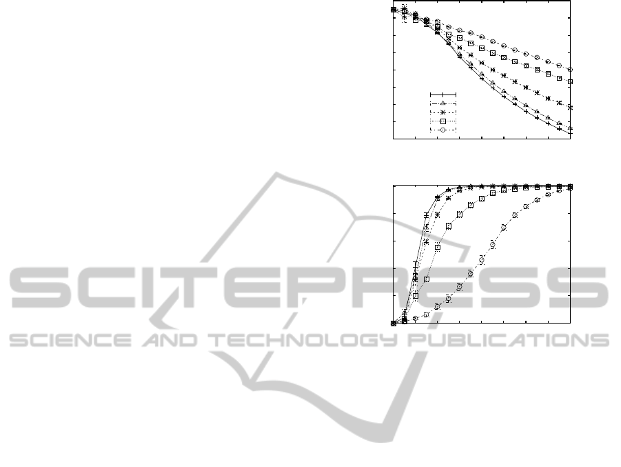
landscape. Figure 1 shows the average adaptive walk

length (top plot) and the average number of unique

(local) optimal solutions (bottom plot). In essence,

this ﬁgure shows that increasing K reduces the aver-

age length of an adaptive walk, i.e. the landscapes

becomes more rugged, and at the same time increases

the probability that the EA gets trapped at a new local

optimal solution. On the other hand, increasing α re-

duces the ruggedness of the ﬁtness landscapes and de-

creases the number of unique local optimal solutions.

As is apparent from the ﬁgure, the parameters K and

0 2 4 6 8 10 12 14 16

Average adaptive walk length

#Neighbors K

α=0.0

α=0.5

α=1.0

α=1.5

α=2.0

2000

4000

6000

8000

10000

0 2 4 6 8 10 12 14 16

Average number of unique local

optimal solutions found

#Neighbors K

Figure 1: Plots showing the average length (top) and the av-

erage number of unique local optimal solutions found (bot-

tom) across 10 repetitions of 10000 adaptive walks for dif-

ferent neighborhood sizes K and model parameter values α.

α allow us to cover a reasonable mixture of ﬁtness

landscapes exhibiting different topologies or levels of

ruggedness and epistasis.

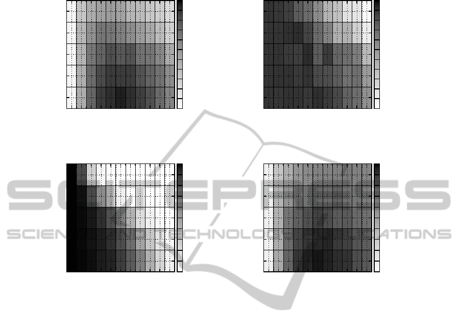
Figure 2 shows how a lethal optimization scenario

affects the best solution ﬁtness found (top plots) and

the (remaining) population size (bottom left plot) for

TGA with a rather traditional setup (TS = 2, p

= 0.0

and Poisson mutation with p

= 1/N) as a function

of the parameters K and α; the bottom right plot in-

dicates the scope available for optimization after the

initialization of the population. From the top plots we

can see that the performance is most affected for ﬁt-

ness landscapes that are rugged (large K) but contain

some structure in the sense that some solution bits are

more important than others (large α). As is apparent

from the bottom left plot, the reason for this pattern is

that the population size at the end of the optimization

decreases as K and/or α increase, i.e. lethal solutions

are here more likely to be encountered. In fact, for

large K and α, the optimization terminates on average

after only about 25 generations (out of 200). The rea-

son that the population size reduces for large K is that

the ﬁtness landscape becomes more rugged, which in-

creases the risk of evaluating lethal solutions despite

them being located close to high-quality solutions.

Although an increase in α introduces more structure

into the ﬁtness landscape, it has also the effect that so-

EVOLUTIONARY SEARCH IN LETHAL ENVIRONMENTS

TGA - Average best solution fitness

obtained in lethal environment

0 1 2 3 4 5 6 7 8 9 10

#Neighbors K

0.5

1.5

Model parameter α

0.66

0.67

0.68

0.69

0.7

0.71

0.72

0.73

0.74

0.75

0.76

0.77

TGA - Average absolute difference between

the best solution fitness found in

a lethal and non-lethal environment

0 1 2 3 4 5 6 7 8 9 10

#Neighbors K

0.5

1.5

Model parameter α

-0.05

-0.045

-0.04

-0.035

-0.03

-0.025

-0.02

-0.015

-0.01

-0.005

0.005

TGA - Survived proportion of the population

at generation G=200, or µ

/µ

0 1 2 3 4 5 6 7 8 9 10

#Neighbors K

0.5

1.5

Model parameter α

0.1

0.2

0.3

0.4

0.5

0.6

0.7

0.8

0.9

TGA - Average absolute difference between

the best solution fitness found in a non-lethal

environment and the lethal fitness threshold

0 1 2 3 4 5 6 7 8 9 10

#Neighbors K

0.5

1.5

Model parameter α

0.14

0.15

0.16

0.17

0.18

0.19

0.2

0.21

0.22

0.23

0.24

Figure 2: Plots showing the average best solution ﬁtness found by TGA (using TS = 2, p

= 0.0 and Poisson mutation with

= 1/N) in a lethal environment (top left), the average absolute difference between this ﬁtness and the ﬁtness achieved

in a non-lethal environment, i.e. f

LFT

= 0 (top right), the average proportion of the population that survived at generation

G = 200, or µ

/µ

(bottom left), and the average absolute difference between the best solution ﬁtness found and the lethal

ﬁtness threshold in a non-lethal environment (bottom right), on NKα landscapes as a function of the neighborhood size K and

the model parameter α.

lutions which havesome of these important bits set in-

correctly are more likely to be poor. A plausible alter-

native explanation for the poor performance at large

α may be that the lethal ﬁtness threshold is very close

to the best solution ﬁtness that can be found, thus re-

ducing the scope of optimization possible and causing

many solutions to be lethal; the bottom right plot rules

this explanation out. Regarding the (remaining) pop-

ulation size, a greater selection pressure, i.e. a larger

tournament size, can help to maintain a large popula-

tion size for longer, particularly for large K and small

α. On the other hand, being more random in the solu-

tion generation process by using, for example, a larger

mutation and/or crossover rate, has the opposite ef-

fect, i.e. the population size decreases more quickly.

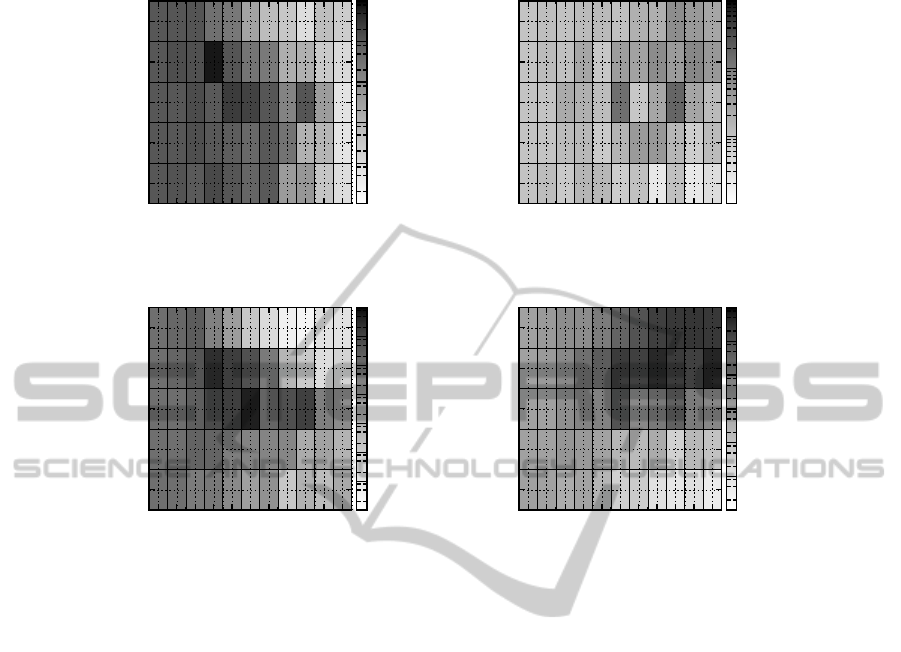
The effect on the (remaining) population size

translates into an impact on the average best solution

ﬁtness. In fact, from Figure 3, we can see that, for

rugged landscapes with structure (i.e. in the range

K > 5, α > 1), TGA is outperformed by a GA with

a rather traditional setup and a PHC in a non-lethal

optimization scenario (right plots) but performs bet-

ter than both algorithms in a lethal optimization sce-

nario (left plots). In fact, as we will also see later, in

the range K > 5, α > 1, PHC performs best among all

the search algorithms considered in the non-lethal en-

vironment but worst in the lethal environment. The

poor performance of PHC in this range is due to the

fact that the hill-climbers in the population are search-

ing the ﬁtness landscape independently of each other.

This may be an advantage in a non-lethal environment

because it can help to maintain diversityin the popula-

tion and prevent premature convergence. However, in

a lethal environment, uncontrolleddiversity is rather a

drawback as it increases the probability of generating

solutions with genotypes that are signiﬁcantly differ-

ent from the ones in the population, which in turn in-

creases the probability of generating lethal solutions.

The less diverse and random optimization of TGA is

also the reason that it outperforms a GA with a more

ECTA 2011 - International Conference on Evolutionary Computation Theory and Applications

Ratio P(f(x) > f

TGA

)/P(f(x) > f

TGA,TS=2,p

=0.0,p

=1/N

lethal optimization

0 1 2 3 4 5 6 7 8 9 10

#Neighbors K

0.5

1.5

Model parameter α

-4

-3

-2

-1

Ratio P(f(x) > f

TGA

)/P(f(x) > f

PHC

lethal optimization

0 1 2 3 4 5 6 7 8 9 10

#Neighbors K

0.5

1.5

Model parameter α

-5

-4

-3

-2

-1

Ratio P(f(x) > f

TGA

)/P(f(x) > f

TGA,TS=2,p

=0.0,p

=1/N

non-lethal optimization

0 1 2 3 4 5 6 7 8 9 10

#Neighbors K

0.5

1.5

Model parameter α

-1

Ratio P(f(x) > f

TGA

)/P(f(x) > f

PHC

non-lethal optimization

0 1 2 3 4 5 6 7 8 9 10

#Neighbors K

0.5

1.5

Model parameter α

-3

-2

-1

Figure 3: (Top) Plots comparing the relative performance of TGA (default parameters) and TGA with TS = 2, p

= 0.0, p

1/N, in a lethal (top left) and non-lethal environment (top right). Darker shades indicate that TGA with TS = 2, p

= 0.0, p

1/N performs better. (Bottom) Plots comparing the relative performance of TGA and PHC (both using default parameters) in a

lethal (bottom left) and non-lethal environment (bottom right). Darker shades indicate that PHC performs better. Performance

is plotted as a function of K and α in all cases. Relative performance is calculated as P( f(x) > f

)/P( f (x) > f

) where P is a

sample probability estimated from 10000 samples and f (x) is a random draw from the search space, while f

and f

represent

the best ﬁtness obtained by the two algorithms.

traditional setup on rugged landscapes with structure.

Let us now analyze how the search algorithms

fare with different parameter settings. Table 2 shows

the average best solution ﬁtness obtained by different

algorithm setups in a lethal and non-lethal environ-

ment (values in parenthesis) on NKα landscapes with

K = 4,α = 2.0 (top table) and K = 10,α = 2.0 (bot-

tom table), respectively. Note that due to the nature

of NKα landscapes (particularly due to the absence of

plateaus or neutral networks in the landscapes), there

was only a single best solution in the population at

each generation. For RBS, this has the effect that

the performance is independent of the crossover rate

because crossover is applied to identical solutions.

The two tables largely conﬁrm the observation made

above: while a relatively high degree of population

diversity and randomness in the solution generation

process may be beneﬁcial in a non-lethal environment

(which is particularly true for rugged landscape as can

be seen from the bottom table), it is rather a draw-

back in a lethal environment as it may increase the

risk of generating lethal solutions and subsequently

limit the effectiveness of evolutionary search. More

precisely, for a lethal environment, the tables indicate

that one should use a GA instead of a PHC, and re-

duce randomness in the solution generation process

by avoiding crossover (generally), and using constant

mutation as well as a relatively large tournament size.

The poor performance of Poisson mutation, which is

a typical mutation mode for GAs, is related to situa-

tions where an over-averaged number of solution bits

is ﬂipped at once. Such variation steps lead to off-

spring that are located in the search space far away

from their non-lethal parents, which can in turn in-

crease the probability of generating lethal solutions.

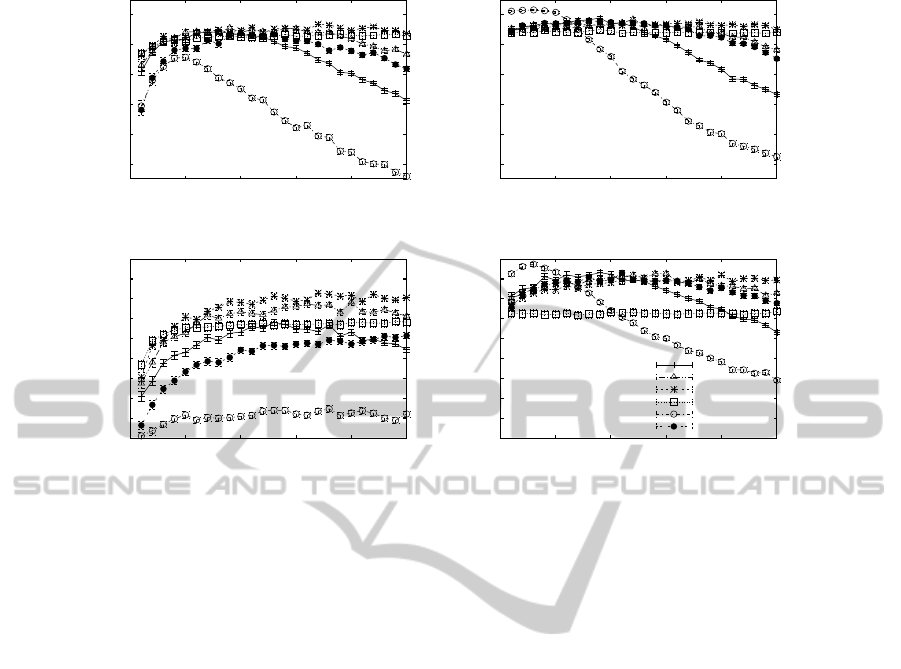
Finally, Figure 4 analyzes whether evolving a

large set of entities for a small number of genera-

tions yields better performance than evolving only a

few entities for many generations; i.e. how is the

trade-off between the initial population size µ

and

the maximum number of generations G. For a non-

lethal environment (right plots), we make two obser-

EVOLUTIONARY SEARCH IN LETHAL ENVIRONMENTS

Table 2: The table shows the average best solution ﬁtness found in a lethal environment after G = 200 generations, and

in parenthesis, the ﬁtness found in a non-lethal environment, for different algorithm setups on K = 4,α = 2.0 (top) and

K = 10,α = 2.0 (bottom); the results of random sampling were obtained by generating G × µ

= 200× 30 = 6000 solutions

per run at random and averaging over the best solution ﬁtness values found. The numbers in the subscript indicate the rank

of the top ﬁve algorithm setups within the respective environment and ﬁtness landscape conﬁguration. We highlighted all

algorithm setups (among the top ﬁve) in bold face that are not signiﬁcantly worse than any other setup. A Friedman test

revealed a signiﬁcant difference between the search algorithm setups in general, but differences among the individual setups

were tested for in a post-hoc analysis using (paired) Wilcoxon tests (signiﬁcance level of 5%) with Bonferroni correction.

K = 4, α = 2.0

Constant mutation Poisson mutation

d = 1 d = 2 p

= 0.5/N p

= 1.0/N

TGA

TS = 1

= 0.0 0.722

(0.7297

) 0.6998 (0.7286) 0.7174 (0.7272) 0.7141 (0.7285)

= 0.25 0.7188 (0.7272) 0.6969 (0.7296

) 0.7128 (0.7275) 0.7029 (0.7296)

= 0.5 0.713 (0.7279) 0.6901 (0.7287) 0.7091 (0.7276) 0.7078 (0.7277)

TS = 2

= 0.0 0.7223

(0.7269) 0.7053 (0.7287) 0.7198 (0.7271) 0.7175 (0.7275)

= 0.25 0.7217 (0.7263) 0.7039 (0.7284) 0.7172 (0.7263) 0.7119 (0.7275)

= 0.5 0.7178 (0.7261) 0.7003 (0.728) 0.7176 (0.7268) 0.7135 (0.727)

TS = 4

= 0.0 0.7218

(0.7266) 0.7107 (0.726) 0.7203 (0.7269) 0.7184 (0.7269)

= 0.25 0.7238

(0.7257) 0.7085 (0.7254) 0.7196 (0.7273) 0.7169 (0.7278)

= 0.5 0.7224

(0.7251) 0.7101 (0.7256) 0.7172 (0.7263) 0.7167 (0.726)

RBS 0.7179 (0.7226) 0.7129 (0.723) 0.7177 (0.7229) 0.7172 (0.7223)

PHC 0.7117 (0.7334

) 0.6843 (0.7271) 0.7033 (0.7343

) 0.6912 (0.7329

)

Random sampling 0.6197 (0.6358)

K = 10,α = 2.0

Constant mutation Poisson mutation

d = 1 d = 2 p

= 0.5/N p

= 1/N

TGA

TS = 1

= 0.0 0.6918 (0.7317) 0.6637 (0.7383

) 0.6812 (0.7338) 0.6767 (0.7356

)

= 0.25 0.6752 (0.7324) 0.6546 (0.7332) 0.6623 (0.7299) 0.6578 (0.7324)

= 0.5 0.6653 (0.7298) 0.6472 (0.7331) 0.6478 (0.7264) 0.6472 (0.7287)

TS = 2

= 0.0 0.702

(0.7299) 0.6697 (0.7318) 0.6938 (0.7307) 0.6821 (0.7305)

= 0.25 0.6897 (0.7277) 0.662 (0.732) 0.6717 (0.7281) 0.6643 (0.7302)

= 0.5 0.6768 (0.7288) 0.6537 (0.7296) 0.6607 (0.7263) 0.659 (0.7274)

TS = 4

= 0.0 0.7072

(0.7275) 0.677 (0.7294) 0.6981

(0.7302) 0.6902 (0.7272)

= 0.25 0.6979 (0.7294) 0.6701 (0.7298) 0.6834 (0.7279) 0.6805 (0.7263)

= 0.5 0.6936 (0.7265) 0.6635 (0.7296) 0.6715 (0.7258) 0.67 (0.7255)

RBS 0.7102

(0.7207) 0.6871 (0.7219) 0.7056

(0.7217) 0.6987 (0.7215)

PHC 0.6651 (0.7434

) 0.6476 (0.7345) 0.6568 (0.7438

) 0.6517 (0.7421

)

Random sampling 0.632 (0.6524)

vations: (i) best performance is achieved with PHC

using a rather small population size of about µ

= 30,

and (ii) for population sizes µ

> 50 one should use a

GA whereby the applied tournament size or selection

pressure should increase with the population size. As

the population size increases, the maximum number

of generations G available for optimization is simply

insufﬁcient for PHC or a GA with low selection pres-

sure and/or much randomness in the solution genera-

tion process to converge quickly to a high-quality part

of the search space. However, on the other hand, a

GA with too much selection pressure may cause the

population to get stuck at local optima, especially on

rugged ﬁtness landscapes (see result of RBS in the

bottom right plot). In a lethal optimization scenario

(left plots), a GA clearly outperforms PHC (regard-

less of the population size) due to the reasons men-

tioned above. Furthermore, unlike to the non-lethal

case, we observe that a GA should use an above-

average large tournament size already for small popu-

lation sizes of µ

> 30. Similar to the non-lethal case,

however, there is a saturation point with RBS, beyond

which a further increase in the population size has no

effect (see e.g. bottom left plot).

4 SUMMARY AND

CONCLUSIONS

This paper has conducted an initial investigation of

the impact of lethal solutions (here modeled as candi-

ECTA 2011 - International Conference on Evolutionary Computation Theory and Applications

0.67

0.68

0.69

0.7

0.71

0.72

0 50 100 150 200 250

Average best solution fitness

Initial population size µ

K=4, α=2.0, lethal optimization

0.67

0.68

0.69

0.7

0.71

0.72

0 50 100 150 200 250

Average best solution fitness

Initial population size µ

K=4, α=2.0, non-lethal optimization

0.66

0.67

0.68

0.69

0.7

0.71

0.72

0.73

0.74

0.75

0 50 100 150 200 250

Average best solution fitness

Initial population size µ

K=10, α=2.0, lethal optimization

0.66

0.67

0.68

0.69

0.7

0.71

0.72

0.73

0.74

0.75

0 50 100 150 200 250

Average best solution fitness

Initial population size µ

K=10, α=2.0, non-lethal optimization

TGA, TS=1

TGA, TS=2

TGA, TS=4

RBS

PHC

TGA, TS=2,p

=0.0,p

=1/N

Figure 4: Plots showing the average best solution ﬁtness obtained by different search algorithms in a lethal environment (left)

and non-lethal environment (right) on NKα landscapes with K = 4,α = 2.0 (top) and K = 10,α = 2.0 (bottom) as a function

of the initial population size µ

; the maximum number of ﬁtness evaluations available for optimization was ﬁxed at 6000

(corresponding to the default setting G = 200,µ

= 30), i.e. G = ⌊6000/µ

⌋. If not otherwise stated, an algorithm used a

constant mutation mode with d = 1 and no crossover, i.e. p

= 0.0.

date solutions below a certain ﬁtness threshold) on

evolutionary search. In essence, the effect of evaluat-

ing a lethal solution is that the solution is immediately

removed from the population and the population size

is reduced by one. This kind of scenario can be found

in Natural evolution, where the presence of lethal mu-

tants may promote robustness over evolvability, but it

is also a characteristic of certain closed-loop evolu-

tion applications, for example, in autonomous robots

or nano-technologies. When faced with this kind of

scenario in optimization, the challenge is to discover

innovative and ﬁt candidate solutions without reduc-

ing the population too rapidly.

Our analysis has been focused on the following

three main aspects: (i) analyzing the impact of lethal

solutions on a standard evolutionary algorithm (EA)

framework, (ii) determining challenging ﬁtness land-

scape topologies in a lethal environment, and (iii) tun-

ing EAs to perform well within a lethal optimiza-

tion scenario. Generally, the presence of lethal so-

lutions can affect that performance of EAs, but the

largest (negative) impact was observed for ﬁtness

landscapes that are rugged and possess some struc-

ture in the sense that some solution bits are more im-

portant than others; in terms of our test functions,

which were NKα landscapes, this type of landscape

corresponds to large values of K and α. For this

ﬁtness landscape topology, we obtained best perfor-

mance in a non-lethal environment using a small pop-

ulation of stochastic hill-climbers. In a lethal environ-

ment, however, signiﬁcantly better results were ob-

tained using an EA that limits randomness in the so-

lution generation process by employing elitism, a rel-

atively large selection pressure, a constant mutation

mode (i.e. ﬂipping exactly one solution bit as op-

posed to ﬂipping each bit independently with some

low probability), and no or a small crossover rate.

Also, in a lethal optimization scenario, we observed

that an EA that evolves a large set of entities (e.g. au-

tonomous robots or software) for a small number of

generations performs better than one that evolves a

few entities for many generations. The practical im-

plication of this is that, if possible, a larger budget

should be allocated for the production of the entities

in the ﬁrst place rather than for attempting to prolong

the testing or optimization phase.

5 FUTURE WORK

Our study has of course been very limited, and there

remains much else to learn about optimization prob-

lems subject to lethal solutions and search policies

EVOLUTIONARY SEARCH IN LETHAL ENVIRONMENTS

for dealing with these problems. Our current re-

search is looking at the design and tuning of intelli-

gent search policies. We have experimented with an

EA that learns ofﬂine, e.g. using reinforcement learn-

ing, when to switch between different selection and

variation operators settings (online) during the opti-

mization (here we used an approach similar to (All-

mendinger and Knowles, 2011)); this EA can yield

better performance than a static or non-learning EA.

It might be worth mentioning that a well-performing

policy learnt ofﬂine by this EA is one that increases

randomness in the solution generation process if and

only if the optimization is in the ﬁnal stages and the

remaining population of reasonable size.

Alternatively to a learning approach, an EA may

be augmented with a strategy that uses assumptions of

local ﬁtness correlation to pre-screen the designs and

forbids the upload of potential lethals. Such a strat-

egy is similar to brood selection with repair and/or

some ﬁtness approximation schemes used in EAs to

ﬁlter solutions before evaluation (Walters, 1998; Jin,

2005).

Finally, analyzing the effect of lethal solutions and

search policies on different and perhaps more realis-

tic ﬁtness landscapes than NKα landscapes, e.g. ones

with neutral plateaux, is another avenue we are pur-

suing. In the further future, we might enjoy trying

out our strategies on real lethal environments in au-

tonomous robots, nano-technologies or similar.

REFERENCES

Allmendinger, R. and Knowles, J. (2011). Policy learning

in resource-constrained optimization. In Proceedings

of GECCO, pages 1971–1978.

Barnett, L. (2001). Netcrawling-optimal evolutionary

search with neutral networks. In Proceedings of CEC,

pages 30–37.

Bullock, S. (2003). Will selection for mutational robustness

signiﬁcantly retard evolutionary innovation on neutral

networks? In Artiﬁcial Life VIII, pages 192–201.

Calzolari, D., Bruschi, S., Coquin, L., Schoﬁeld, J., Feala,

J. D., Reed, J. C., McCulloch, A. D., and Paternostro,

G. (2008). Search algorithms as a framework for the

optimization of drug combinations. PLoS Computa-

tional Biology, 4:1.

Ciuti, G., Donlin, R., Valdastri, P., Arezzo, A., Menciassi,

A., Morino, M., and Dario, P. (2010). Robotic versus

manual control in magnetic steering of an endoscopic

capsule. Endoscopy, 42(2):148–52.

Forrest, S. and Mitchell, M. (1993). Relative building-block

ﬁtness and the building-block hypothesis. In Founda-

tions of Genetic Algorithms 2, pages 109–126.

Harvey, I., Husbands, P., Cliff, D., Thompson, A., and

Jakobi, N. (1996). Evolutionary robotics: The Sussex

approach. Robotics and Autonomous Systems, 20(2-

4):205–224.

Hebbron, T., Bullock, S., and Cliff, D. (2008). NKα:

Non-uniform epistatic interations in an extended NK

model. In Artiﬁcial Life XI, pages 234–241.

Hughes, B. D. (1995). Random walks and random environ-

ments. Clarendon Press.

Jin, Y. (2005). A comprehensive survey of ﬁtness approxi-

mation in evolutionary computation. Soft Computing,

9(1):3–12.

Kauffman, S. (1989). Adaptation on rugged ﬁtness land-

scapes. In Lecture Notes in the Sciences of Complex-

ity, pages 527–618.

Klockgether, J. and Schwefel, H.-P. (1970). Two-phase noz-

zle and hollow core jet experiments. In Engineering

Aspects of Magnetohydrodynamics, pages 141–148.

Moglia, A., Menciassi, A., Schurr, M. O., and Dario, P.

(2007). Wireless capsule endoscopy: from diagnostic

devices to multipurpose robotic systems. Biomedical

Microdevices, 9(2):235–243.

Rechenberg, I. (2000). Case studies in evolutionary exper-

imentation and computation. Computer Methods in

Applied Mechanics and Engineering, 2-4(186):125–

140.

Schonfeld, J. (2007). A study of mutational robustness as

the product of evolutionary computation. In Proceed-

ings of GECCO, pages 1404–1411.

Shir, O. M., Emmerich, M., B¨ack, T., and Vrakking, M.

J. J. (2007). The application of evolutionary multi-

criteria optimization to dynamic molecular alignment.

In Proceedings of CEC, pages 4108–4115.

Small, B. G., McColl, B. W., Allmendinger, R., Pahle,

J., L´opez-Castej´on, G., Rothwell, N. J., Knowles, J.,

Mendes, P., Brough, D., and Kell, D. B. (2011). Ef-

ﬁcient discovery of anti-inﬂammatory small molecule

combinations using evolutionary computing. Nature

Chemical Biology, (to appear).

Syswerda, G. (1989). Uniform crossover in genetic algo-

rithms. In Proceedings of ICGA, pages 2–9.

Thompson, A. (1996). Hardware Evolution: Automatic de-

sign of electronic circuits in reconﬁgurable hardware

by artiﬁcial evolution. PhD thesis, University of Sus-

sex.

Walters, T. (1998). Repair and brood selection in the travel-

ing salesman problem. In Proceedings of PPSN, pages

813–822.

Watson, R. A., Ficici, S. G., and Pollack, J. B. (2002). Em-

bodied evolution: Distributing an evolutionary algo-

rithm in a population of robots. Robotics and Au-

tonomous Systems, 39(1):1–18.

Zykov, V., Mytilinaios, E., Adams, B., and Lipson,

H. (2005). Self-reproducing machines. Nature,

435(7039):163–164.

ECTA 2011 - International Conference on Evolutionary Computation Theory and Applications