
GRAPHICAL MODELS FOR RELATIONS
Modeling Relational Context
Volker Tresp
1,2
, Yi Huang
1
, Xueyan Jiang
2
and Achim Rettinger
3
1
Siemens AG, Corporate Technology, Munich, Germany
2
Ludwig-Maximilians-Universit¨at M¨unchen, Munich, Germany
3
Karlsruhe Institute of Technology, Karlsruhe, Germany
Keywords:
Relational learning, Probabilistic relational models, Relational context information, Recommendation
systems, Graphical models.
Abstract:
We derive a multinomial sampling model for analyzing the relationships between two or more entities. The
parameters in the multinomial model are derived from factorizing multi-way contingency tables. We show
how contextual information can be included and propose a graphical representation of model dependencies.
The graphical representation allows us to decompose a multivariate domain into interactions involving only a
small number of variables. The approach formulates a probabilistic generative model for a single relation. By
construction, the approach can easily deal with missing relations. We apply our approach to a social network
domain where we predict the event that a user watches a movie. Our approach permits the integration of both
information about the last movie watched by a user and a general temporal preference for a movie.
1 INTRODUCTION
In this paper we address the problem of predict-
ing the existence of a relation between two or more
entities. Examples would be relations describing
the interest of a user for items, e.g., watches(User,
Movie), friendship relations in a social network, e.g.,
isFriendsWith(PersonA, PersonB), or patient treat-
ment and patient diagnosis relations in a clinical
setting, e.g., getsTreatment(Patient, Treatment), has-
Disease(Patient, Disease). Although a number of
different approaches have been proposed for this
task (Koller and Pfeffer, 1998; Taskar et al., 2002;
Getoor et al., 2007; Domingos and Richardson, 2007;
Kemp et al., 2006; Xu et al., 2006), matrix factor-
ization approaches are clearly among the leading ap-
proaches since they can readily exploit structure in
relational patterns. For relations with an arity larger
than two, tensor factorization recently have become
popular, enabling the modeling of relations such as
rates(User, Movie, Rating) or watches(User, Movie,
May2011) (Rendle et al., 2010). In most cases, ma-
trix and tensor factorization have been implemented
in a deterministic interpretation, e.g., simply to com-
plete a matrix or a tensor based on a low-rank approx-
imation. Exception are the probabilistic approaches
in (Yu et al., 2006; Chu et al., 2006; Salakhutdi-
nov and Mnih, 2007) where Gaussian models and
Bernoulli models are employed to model preferences
of users for certain items. Here we show that by as-
suming a particular sampling scheme and by normal-
izing the factorized matrix and the factorized tensor,
respectively, we can obtain a probabilistic interpreta-
tion in terms of a multinomial model. In particular,
we assume that a statistical unit or a data point —
and thus also a row in the data matrix— is defined
by a relational tuple, i.e. an instantiated relation. As
an example, let a data point be defined by the ob-
servation that a particular user u watches a particular
movie m, let C be the contingency table of observed
user/movie pairs, and let
ˆ
C be the factorized and nor-
malized contingency table. Then we would estimate
that
ˆ
P(u, m) = ˆc
u,m
, where ˆc
u,m
= {
ˆ
C}
u,m
. An advan-
tage of this approach is that we only model what is
observed, which means that we do not need to em-
ploy a missing data mechanism for unobserved re-
lations. This is particulary useful in the typical sit-
uation where only positive examples for a relation
are available. In many other approaches one needs
to specify if a relational instance not present in the
data should be assumed missing or non-existent. If
modeled as missing, potentially complex missing data
mechanism need to be applied.
Another advantage is that we now can extend the
114
Tresp V., Huang Y., Jiang X. and Rettinger A..
GRAPHICAL MODELS FOR RELATIONS - Modeling Relational Context.
DOI: 10.5220/0003665201140120
In Proceedings of the International Conference on Knowledge Discovery and Information Retrieval (KDIR-2011), pages 114-120
ISBN: 978-989-8425-79-9
Copyright
c
2011 SCITEPRESS (Science and Technology Publications, Lda.)

model with contextual information. Let’s consider the
relation watches(User, Movie, LastMovieWatched-
ByUser, Month) which says that a user watches a
movie in a given month and where we also have infor-
mation about the last movie that the user has watched.
Such a relation can be modeled by a four-way tensor
which would give us, after reconstruction and normal-
ization,
ˆ
P(User, Movie, LastMovieWatchedByUser,
Month). Naturally, the contingency tables for ten-
sors are very sparse, in particular if one considers
that the involved variables often have many thousand
states; the goal of this paper is to exploit structure in
the data, visualized as graphical models, to generate
data-efficient models. Graphical models are a com-
mon approach for exploiting independencies in high-
dimensional domains.
We believe that this new way of the application of
graphical model can lead to quite interesting and pow-
erful models. A particular benefit is the modularity of
the approach which permits a separate optimization of
local models, which, of course, is the benefit of graph-
ical models —in particular of Bayesian networks and
decomposable models— in general (Lauritzen, 1996).
The paper is organized as follows. In the next sec-
tion, we describe related work. In Section 3 we de-
scribe the basic idea and in Section 4 we develop the
approach using data from a social network. We show
that contextual information can improve the predic-
tion. Section 5 contains our conclusions.
2 RELATED WORK
Graphical models have a long history in expert
systems and statistical modeling (Lauritzen, 1996).
Graphical models have also been applied to relational
domains. Prominent examples are Probabilistic Re-
lational Models (Koller and Pfeffer, 1998; Getoor
et al., 2007), Markov Logic Networks (Domingos and
Richardson, 2007), and Infinite Hidden Relational
Models (Kemp et al., 2006; Xu et al., 2006). Al-
though being very general, the application of these
models to a given relational domain might still be
tricky: Probabilistic Relational Models require in-
volved structural optimization, Markov Logic Net-
works depend on the available of rule sets and logical
expressions (approximately) valid in the domain and
Infinite Hidden Relational Models require complex
inference processes. Here, we focus on the modeling
of a single relation which leads to simpler and scal-
able models. The sampling assumptions in this paper
are similar to the ones made in the pLSI model (Hof-
mann, 1999) and the underlying assumptions in some
matrix and tensor decomposition approaches (Ren-
dle et al., 2010; Wermser et al., 2011), although in
these papers, this sampling assumption is not stated
explicitly. The difference is that here we exploit inter-
dependencies in the domain using graphical models
whereas those approaches form a joint clustering and
factorization model, respectively. It might be inter-
esting to note that (Rendle et al., 2010) uses a simpli-
fied factorized model which consists of sums of terms
defined for individual interactions whereas we obtain
products of simple interaction components. The ar-
gument that higher-order tensor models permit the in-
tegration of contextual background information was
also made in (Wermser et al., 2011).
There is a large literature on matrix completion
methods, which we apply to model the interactions
in the graphical model (Cands and Recht, 2008). In
particular, the winning entry to the NETFLIX com-
petition used matrix completion approaches (Takacs
et al., 2007; Bell et al., 2010). Tensor factoriza-
tion has become an area of growing interest. A re-
cent overview has been provided in (Kolda and Bader,
2009).
In (Yu et al., 2006; Salakhutdinov and Mnih,
2007) contextual information was included in matrix
completion approaches. A Gaussian noise model is
employed which is more suitable for modeling contin-
uous and ordinal quantities, such as a user score for a
movie, than for the likelihood of the existence of a re-
lation, as we are doing here. Also, those approaches
often have difficulties in situations where only posi-
tive examples for a relation are available; they need to
distinguish between true negatives (e.g., it is known
that a user does not like a movie) and missing in-
formation (e.g., it is unknown if a user likes a par-
ticular movie). Bernoulli and Gaussian sampling ap-
proaches have been pursued in (Chu et al., 2006; Chu
and Ghahramani, 2009).
3 RELATIONAL POPULATIONS,
GRAPHICAL STRUCTURES,
AND THE MULTINOMIAL
MODEL
In this section we describe the standard object-
centered sampling model and contrast it with the
relation-oriented sampling model used in this paper.
3.1 Standard Object-oriented Sampling
Assumption
Traditionally, statistical units, i.e. data points, are
associated with objects and statistical models con-
GRAPHICAL MODELS FOR RELATIONS - Modeling Relational Context
115

……………
1001
U2
1011
U1
I4I3I2I1
………
I4U2
ID3
I2U1
ID2
I1U1
ID1
IU
Figure 1: Left: In a more traditional view, each row is
defined by a user and the columns represent the different
items. A one indicates that a user has purchased an item.
Right: Each row is defined by an event user-buys-item,
which is the sampling assumption used in this paper.
cern the statistical dependencies between attributes of
those objects. A typical example is a medical do-
main where one analyzes the dependencies between
the attributes of a population of patients, for exam-
ple in form of a Bayesian network. In a data matrix
the patients would define the rows and would act as a
unique identifiers and the attributes would define the
columns. A fundamental task is then to predict if a
novel object belongs to the same population (density
estimation), or what values a variable has to assume
such that the likelihood that the object belongs to the
same population is maximized (predictive modeling).
This approach is also quite common in modeling
relational domains. For example, one might analyze
the preferences of a population of U users based on
user attributes and based on known preferences for I
items, e.g., buy(User, Item), where the preferences are
essentially also treated as attributes of the users (Fig-
ure 1, Left). In (Breese et al., 1998) a Bayesian net-
work is described where a binary node x
j
represents
an item and the state of the node indicates if a user has
bought an item (x
j
= 1) or not (x
j
= 0). The Bayesian
network models then
ˆ
P(x
1
, . . . , x
I
). (1)
A problem one encounters in these models is that
one needs to distinguish between relationships known
not to exist and relations that are unknown. For ex-
ample, in the Bayesian networks in (Breese et al.,
1998) and in the Dependency Networks (Heckerman
et al., 2000) missing relations are treated as not-to-
exist whereas in (Koller and Pfeffer, 1998; Xu et al.,
2006; Domingos and Richardson, 2007; Getoor et al.,
2007) Gibbs sampling and loopy belief propagation
are used for dealing with unknown relationships.
3.2 Relation-oriented Sampling
Assumption
In our relation-oriented view, an instance is defined
by an observed relation, i.e., a tuple, typically describ-
ing the relationship between two or more objects (Fig-
ure 1, Right). The population then consists of all true
tuples and a sample is a random subset of those true
tuples. Thus, whereas in the previous subsection we
assumed that either users or items define the rows in
the data matrix, here we assume that each observed
instantiated relation (tuple) defines a row.
Considering again the relation buy(User, Item), the
data matrix would contain two columns encoding the
user and the item, respectively, and a model would
estimate
ˆ
P(User = u, Item = i). (2)
Note that whereas Equation 1 describes a probability
distribution over I binary variables, this equation de-
scribes a multinomial model with two variables where
the two variables have U and I states, respectively.
Considering now that we generalize from two to A
attributes that describe a relation, i.e., are informative
for determining the existence of a relation, the basic
problem is to evaluate P(x
1
, . . . , x
A
), i.e., the probabil-
ity that a novel relationship with attributes x
1
, . . . , x
A
is likely to exist. Alternatively, it might be interesting
to predict the most likely value of one of the attributes
given other attributes, such as P(x
1
|x
2
, . . . , x
A
), e.g.,
the probability of an item x
1
given a user x
2
and given
contextual information x
3
, . . . , x
A
.
In object-to-object relationships, variables typi-
cally contain many states and a contingency table in-
volving all variables can be very sparse. In high-
dimensional domains graphical models have been
quite effective in the past (Lauritzen, 1996) and so
in this paper we will apply them as well. As dis-
cussed earlier, the novelty in this paper is that we ap-
ply graphical models in domains where the relations
form the instances and where we model just a sin-
gle relation instead of a whole network of entities and
their relationships.
For our purpose, Bayesian networks and decom-
posable models are most suitable. For a Bayesian net-
work model, the probability distribution factors as
P(x
1
, . . . , x
A
) =
A
∏
i=1
P(x
i
|par(x
i
))
=
A
∏
i=1
P(x
i
, par(x
i
))
P(par(x
i
))
.
Typically a Bayesian network is depicted as a di-
rected graphical model without directed loops. In this
model, par(x
i
) denotes the direct parents of x
i
.
Given a Bayesian network structure, the task
is then to model P(x
i
|par(x
i
)), or equivalently,
P(x
i
, par(x
i
)). If the involved variables have many
states, matrix and tensor completion methods have
been successful in the past and we also apply those
in our approach, as described in the next Section.
KDIR 2011 - International Conference on Knowledge Discovery and Information Retrieval
116

4 DEVELOPMENT OF A
CONCRETE MODEL USING
DATA FROM THE GETGLUE
SOCIAL NETWORK SITE
4.1 GetGlue: A Social Network Site
We based our experiments on GetGlue
(http://getglue.com), a social network that lets
users connect to each other and share Web navigation
experiences. In addition, GetGlue uses semantic
recognition techniques to identify books, movies,
and other similar topics and publishes them in the
form of data streams. Users can observe the streams
and receive recommendations on interesting findings
from their friends. Both the social network data
and the real-time streams are accessible via Web
APIs. Users have online names, and they know
and follow other users using well-known Semantic
Web vocabularies, such as the Friend of a Friend
(FOAF) vocabulary for user names and the knows
relationship, and the Semantically Interlinked Online
Communities (SIOC) for the follows relationship.
Objects represent real-world entities (such as movies
or books) with a name and a category. Resources
represent information sources that describe the actual
objects, such as webpages about a particular movie
or book.
In the following we use GetGlue data for recom-
mending items, in particular movies, to users. This is
essentially a probability density estimation problem
since we estimate the probability that a novel user-
movie pair belongs to the population.
4.2 Modeling User-movie Events
We model the event that a user watches a movie. The
graphical model consists of two attributes, i.e., the
user and the movie (Figure 2). The rows in the data
matrix are then defined by known user-movie events
and the columns consists of two variables with as
many states as there are users and movies, respec-
tively. A contingency table C is formed. Entry c
u,m
counts how often user u has watched movie m. By
dividing the entries by the overall counts, we can in-
terpret the entries as estimates for the probabilities
of observing a user-movie pair under this sampling
assumption, i.e. as a maximum likelihood estimate
of P(u, m). This matrix will contain many zero en-
tries and the maximum likelihood estimates are noto-
riously unreliable. We follow common practice and
smooth the matrix using a matrix factorization ap-
proach. We perform a singular value decomposition
M
U
Figure 2: A graphical model for the dependencies between
users U and movies M.
CC
T
= U DU
T
and obtain the low-rank approxima-
tion (Huang et al., 2010)
ˆ
C = U
s
diag
s
d
l
d
l
+ λ
U
⊤
s
C
where diag
s
d
l
d
l
+λ
is a diagonal matrix containing
the s leading eigenvalues in D and where U
s
contains
the corresponding s columns of U. λ is a regulariza-
tion parameter. After proper normalization
ˆ
C, the en-
tries can be interpreted as
ˆ
P(u, m), i.e., an estimate of
the probability of observing the relation that user u
watches movie m.
1
It should be noted that matrix completion is an ac-
tive area of research and many other matrix comple-
tion methods are applicable as well. Recommenda-
tions for users can now be based on
ˆ
P(u, m).
4.3 Adding Information on the Last
Movie watched
Certainly, there is a sequential nature of the user-
watches-movie process that the model so far can-
not capture. In particular we might consider the last
movie that a user has watched as additional informa-
tion (Rendle et al., 2010). Note that we now obtain
a truly ternary relation watches(u,m,l) consisting of
user, movie and last movie l watched by the user. The
approach followed in (Rendle et al., 2010) is to con-
sider a three-way contingency table and apply tensor
factorization as a tensor smoothing approach. There
it was argued that general tensor factorization, such
as PARAFAC or Tucker (Kolda and Bader, 2009), are
too difficult to apply in this situation since the con-
tingency table is very sparse and a simplified addi-
tive model is applied. In our approach we suggest
that an appropriate graphical model is shown in Fig-
ure 3 (left).
2
The model indicates that the last movie
1
Normalization takes care that all entries are non-zero
and are smaller than one. Incidentally, this step turns out to
be unnecessary in the regularized reconstruction, since af-
ter matrix completion all entries already obeyed these con-
straints. A second step ensures that the sum over matrix
entries is equal to one.
2
A link from the last movie to movie might appear more
plausible. If one does that change, the link between user
and movie would need to point from movie to user, such
that no collider (more than one link pointing to the same
node) appears. With a collider one would need to use a
tensor model as a local model.
GRAPHICAL MODELS FOR RELATIONS - Modeling Relational Context
117
TimeOf
Watching
M
U
Last
M
U
Last
Figure 3: Left: As additional information, the last movie,
which the user has watched, is added. Right: The month
when the user watches the movie is added.
watched by a user directly influences the next movie
that a user watches but that given that information,
last movie and user are independent. The great advan-
tage now is that we do not need to readapt the user-
movie model but can model independently the movie-
last-movie dependency. Again we calculate empirical
probabilities based on the contingency table, smooth
the table using matrix factorization and obtain
ˆ
P(m, l).
We combine both models and form
ˆ
P(u, m, l) =
ˆ
P(u, m)
ˆ
P(m, l)
ˆ
P(m)
.
Note that in contrast to (Rendle et al., 2010), we do
not obtain a sum of local models but a product of local
models.
4.4 Adding Time of the Event
Next we consider the instance of time when a movie
is watched t. Certainly, the preference for movies
changes in time and at certain instances in time a
movie might be very popular and then decrease in
popularity. Also, a movie can only be watched af-
ter it is released. Time of watching in units of month
is added to the model. Again we formed an empirical
estimate based on the movie-time of watching contin-
gency table. The graphical model is shownin Figure 3
(right).
We now obtain
ˆ
P(u, m, l,t) =
ˆ
P(u, m)
ˆ
P(m, l)
ˆ
P(m,t)
(
ˆ
P(m))
2
.
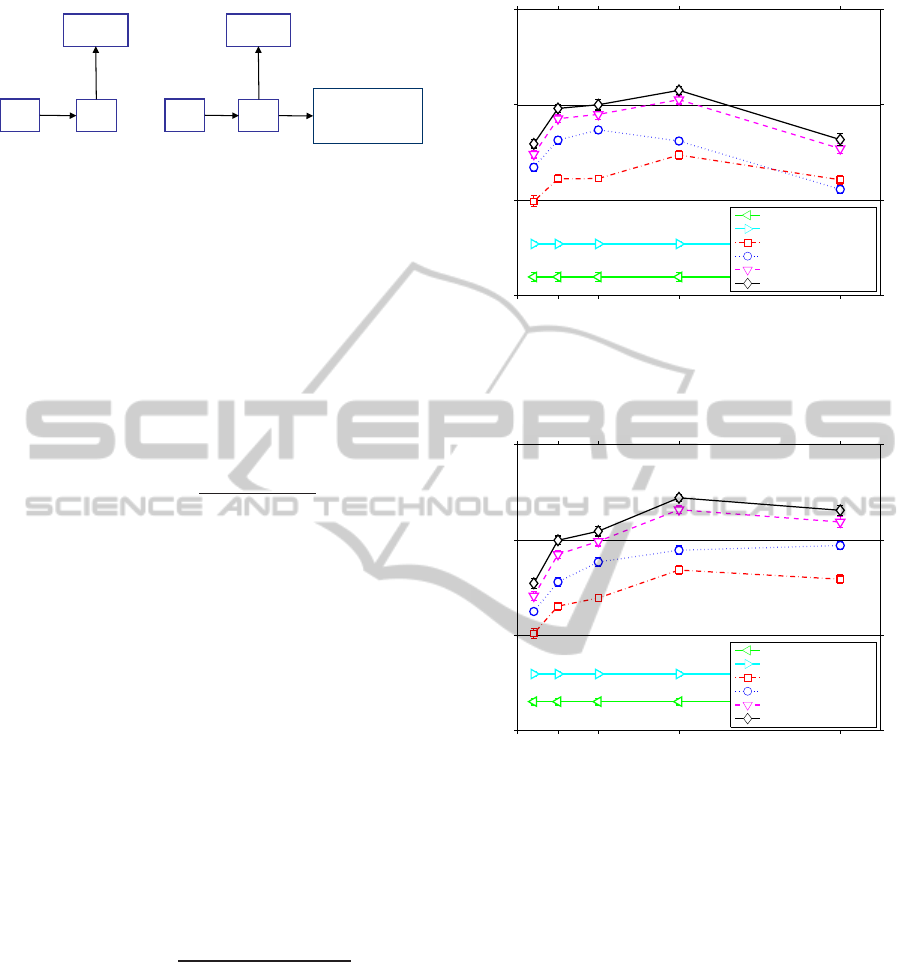
4.5 Experimental Results
In Figures 4 and 5 we see experimental results. The
results are based on 3076 users and 9707 movies and
we considered 44 months. Before smoothing, the
user-movie matrix had 1.8% nonzero entries and the
last movie-movie matrix had 1.21% nonzero entries.
In all experiments, we display the cross-validated
(5 folds) NDCG score (Jarvelin and Kekalainen,
2000) (described in the Appendix) as a function of
the rank s of the approximation. The top plot shows
0 50 100 200 400
0.15
0.2
0.25
0.3
Number of latent variables
NDCG all
Friendship
Movie−Time(MT)
LastMovie−Movie(LM)
User−Movie(UM)
UM + LM
UM + LM + MT
Figure 4: Experiments with social networks data without
model regularization. NDCG score as a function of s, the
rank in the matrix completion.
0 50 100 200 400
0.15
0.2
0.25
0.3
Number of latent variables
NDCG all
Friendship
Movie−Time(MT)
LastMovie−Movie(LM)
User−Movie(UM)
UM + LM
UM + LM + MT
Figure 5: The same model as in Figure 4 but with regular-
ization (λ > 0).
results without regularization (λ = 0) and the bottom
shows a regularized solution. The regularizes solu-
tion shows much better performance and will now
be discussed. MT is the baseline and shows the pre-
dictive performance if movies are simply rated based
in their overall popularity in a given month. LM al-
ready shows much better performance where the pre-
diction is based on information about the last movie
watched. This model purely models the Markov prop-
erty of the event of watching movies. UM shows the
performance based on the classical user-movie model
and is better than the LM model. Thus, personaliza-
tion is more informative than sequence information.
Most interesting, by combining both sources of in-
formation, the performance is greatly improved (UM
+ LM). UM + LM + MT combines the user-movie,
movie-last move and the movie-time model, thus in-
formation about when the movie was watched was in-
KDIR 2011 - International Conference on Knowledge Discovery and Information Retrieval
118
0 50 100 200 400
0.15
0.2
0.25
0.3
Number of latent variables
NDCG all
User−Movie(UM)
UM + LM(avg)
UM + LM + MT(avg)
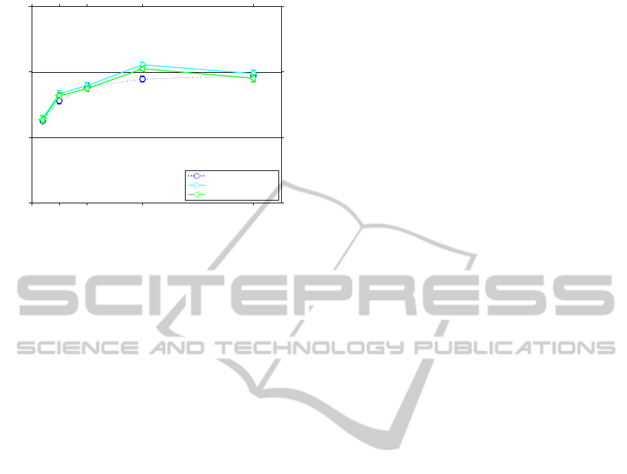
Figure 6: The figure shows results obtained by simply
adding the estimated probabilities for the components.
cluded. The superior performance of the combined
model clearly confirms the benefits of the proposed
approach.
An interesting question is how a simple averaging
of the probabilities of the individual models would
perform. Figure 6 shows that adding the individual
models also improves the performance but that the
gain is better in our approach, based on a multiplica-
tive model.
5 CONCLUSIONS
In this paper we have described a novel approach for
applying graphical models to relational domains. We
define a statistical unit, i.e., instance, by object-to-
object relationships. We applied our approach to a
social network setting and to user-item modeling and
showed that contextual information can be included
to improve prediction accuracy. The great advantage
of the approach is its modularity which permits the
modeling of domains with many variables. Note that
information such as the last movie watched by the
user would be very difficult or impossible to encode
by most other relational learning approaches.
Several extension are possible. First, we used reg-
ularized matrix factorization for approximating the
local probability distributions. Any other of the avail-
able matrix completion approaches could be used as
well (Cands and Recht, 2008), in particular if the
number of objects grows beyond a few thousand. Sec-
ondly, in this paper the local models described inter-
actions between two variables. In case that local inter-
actions between more than two many-state variables
need to be modeled, one can employ tensor factoriza-
tion (Kolda and Bader, 2009) for the local models.
In terms of scalability, the limiting factor is the
matrix completion step but very fast solutions have
recently been proposed (Cands and Recht, 2008).
ACKNOWLEDGEMENTS
We acknowledge funding by the German Federal
Ministry of Economy and Technology (BMWi) under
the THESEUS project and by the EU FP 7 under the
Integrated Project LarKC.
We would like to thank Hendrik Wermser for pro-
viding us with the data set used in the experiments.
REFERENCES
Bell, R. M., Koren, Y., and Volinsky, C. (2010). All together
now: A perspective on the netflix prize. Chance.
Breese, J. S., Heckerman, D., and Kadie, C. (1998). Empir-
ical analysis of predictive algorithms for collaborative
filtering. In Uncertainty in Artificial Intelligence.
Cands, E. J. and Recht, B. (2008). Exact matrix completion
via convex optimization. Computing Research Repos-
itory - CORR.
Chu, W. and Ghahramani, Z. (2009). Probabilistic models
for incomplete multi-dimensional arrays. In AISTATS.
Chu, W., Sindhwani, V., Ghahramani, Z., and Keerthi, S. S.
(2006). Relational learning with gaussian processes.
In NIPS.
Domingos, P. and Richardson, M. (2007). Markov logic: A
unifying framework for statistical relational learning.
In Getoor, L. and Taskar, B., editors, Introduction to
Statistical Relational Learning. MIT Press.
Getoor, L., Friedman, N., Koller, D., Pferrer, A., and Taskar,
B. (2007). Probabilistic relational models. In Getoor,
L. and Taskar, B., editors, Introduction to Statistical
Relational Learning. MIT Press.
Heckerman, D., Chickering, D. M., Meek, C., Rounthwaite,
R., and Kadie, C. M. (2000). Dependency networks
for inference, collaborative filtering, and data visual-
ization. Journal of Machine Learning Research.
Hofmann, T. (1999). Probabilistic latent semantic analysis.
In Uncertainty in Artificial Intelligence (UAI).
Huang, Y., Tresp, V., Bundschus, M., Rettinger, A., and
Kriegel, H.-P. (2010). Multivariate structured predic-
tion for learning on the semantic web. In Proceed-
ings of the 20th International Conference on Inductive
Logic Programming (ILP).
Jarvelin, K. and Kekalainen, J. (2000). IR evaluation meth-
ods for retrieving highly relevant documents. In SI-
GIR’00.
Kemp, C., Tenenbaum, J. B., Griffiths, T. L., Yamada, T.,
and Ueda, N. (2006). Learning systems of concepts
with an infinite relational model. In Poceedings of the
National Conference on Artificial Intelligence (AAAI).
GRAPHICAL MODELS FOR RELATIONS - Modeling Relational Context
119

Kolda, T. G. and Bader, B. W. (2009). Tensor decomposi-
tions and applications. SIAM Review.
Koller, D. and Pfeffer, A. (1998). Probabilistic frame-based
systems. In Proceedings of the National Conference
on Artificial Intelligence (AAAI).
Lauritzen, S. L. (1996). Graphical Models. Oxford Statis-
tical Science Series.
Rendle, S., Freudenthaler, C., and Schmidt-Thieme, L.
(2010). Factorizing personalized markov chains for
next-basket recommendation. In World Wide Web
Conference.
Salakhutdinov, R. and Mnih, A. (2007). Probabilistic matrix
factorization. In NIPS.
Takacs, G., Pilaszy, I., Nemeth, B., and Tikk, D. (2007). On
the gravity recommendation system. In Proceedings
of KDD Cup and Workshop 2007.
Taskar, B., Abbeel, P., and Koller, D. (2002). Discrimina-
tive probabilistic models for relational data. In Uncer-
tainty in Artificial Intelligence (UAI).
Wermser, H., Rettinger, A., and Tresp, V. (2011). Modeling
and learning context-aware recommendation scenar-
ios using tensor decomposition. In Proc. of the Inter-
national Conference on Advances in Social Networks
Analysis and Mining.
Xu, Z., Tresp, V., Yu, K., and Kriegel, H.-P. (2006). Infinite
hidden relational models. In Uncertainty in Artificial
Intelligence (UAI).
Yu, K., Chu, W., Yu, S., Tresp, V., and Xu, Z. (2006).
Stochastic relational models for discriminative link
prediction. In Advances in Neural Information Pro-
cessing Systems 19.
APPENDIX
Details on the NDCG Score
We use the normalized discounted cumulative gain
(NDCG) to evaluate a predicted ranking. NDCG is
calculated by summing over all the gains in the rank
list R with a log discount factor as
NDCG(R) =
1
Z
∑
k
2
r(k)
− 1
log(1+ k)
,
where r(k) denotes the target label for the k-th ranked
item in R, and r is chosen such that a perfect rank-
ing obtains value 1. To focus more on the top-ranked
items, we also consider the NDCG@n which only
counts the top n items in the rank list. These scores
are averaged over all ranking lists for comparison.
KDIR 2011 - International Conference on Knowledge Discovery and Information Retrieval
120
