
BIO-INSPIRED BAGS-OF-FEATURES FOR IMAGE
CLASSIFICATION
Wafa Bel Haj Ali
1
, Eric Debreuve
1
, Pierre Kornprobst
2
and Michel Barlaud
1
1
I3S Laboratory, CNRS / University of Nice-Sophia Antipolis, Sophia Antipolis, France
2
INRIA, Sophia Antipolis, France
Keywords:
Image classification, Feature extraction, Bio-inspired descriptor.
Abstract:
The challenge of image classification is based on two key elements: the image representation and the algorithm
of classification. In this paper, we revisited the topic of image representation. Classical descriptors such as
Bag-of-Features are usually based on SIFT. We propose here an alternative based on bio-inspired features.
This approach is inspired by a model of the retina which acts as an image filter to detect local contrasts. We
show the promising results that we obtained in natural scenes classification with the proposed bio-inspired
image representation.
1 INTRODUCTION
In this paper, we focus on the problem of informa-
tion representation for automatic image categoriza-
tion. The classification task consists in identifying the
category of unlabeled images based on the presence of
some particular visual features. Hence, the analysis of
each image is required to extract relevant information
that best describes its content. This topic is challeng-
ing and more and more studied in the computer vision
community, as illustrated by the ImageNet initiative
and the challenges such as PASCAL.
Many algorithms were implemented for image
classification, and most of them were addressed as
learning problems. Most commonly, they are su-
pervised methods meaning that they make use of
an already annotated training set to learn classifiers
(category boundaries) and subsequently label non-
annotated images. Within this kind of methods,
we find the Support Vector Machine (SVM) (Cortes
and Vapnik, 1995), boosting methods (Schapire and
Singer, 1999) like Adaboost (Freund and Schapire,
1995), or voting procedures like k-nearest neighbors
(k-NN) (Denoeux, 1995) (Piro et al., 2010) (Bel Haj
Ali et al., 2010).
Both global and local descriptors havebeen shown
to be efficient. Gist global feature (Oliva and Tor-
ralba, 2001) for example represents a whole scene in
a unique sparse descriptor, while the scale invariant
feature transform (SIFT) (Lowe, 1999) represents in-
formation localized at keypoints of the image allow-
ing the description of each significant object in the
scene independently. Bag-of-Features (Sivic and Zis-
serman, 2006) is a global representation which de-
scribes the occurrence of relevant visual features in
the image. Each feature is extracted based on a given
type of information, and modeled in a particular way
: for example, SIFT features use local gradient orien-
tations and model them statistically.
In the neurosciences community, there is a grow-
ing tendency to exploit the developments in computa-
tional neuroscience and try to apply them to problems
of computer vision. For example, Thorpe and Van
Rullen (Thorpe and Gautrais, 1998) (Van Rullen and
Thorpe, 2001) proposed coding schemes for informa-
tion transmission which led to the SpikeNet technol-
ogy
1
for image processing (Delorme et al., 1999)
(Thorpe et al., 2004) and specific developments like
motion recognition using bio-inspired models (Esco-
bar et al., 2009).
In this work, we propose a novel image descriptor,
based on the retina model introduced by Van Rullen
and Thorpe (Van Rullen and Thorpe, 2001), to deal
with image categorization. Our features represent in-
formation as analyzed by the human retina. Those
features are extracted in a dense way to cover the
whole image and give precise representations of lo-
cal neighborhoods.
This paper is organized as follows : Section 2 will
present our approach and detail the method used for
1
http://www.spikenet-technology.com/
277
Bel Haj Ali W., Debreuve E., Kornprobst P. and Barlaud M..
BIO-INSPIRED BAGS-OF-FEATURES FOR IMAGE CLASSIFICATION.
DOI: 10.5220/0003663402690273
In Proceedings of the International Conference on Knowledge Discovery and Information Retrieval (KDIR-2011), pages 269-273
ISBN: 978-989-8425-79-9
Copyright
c
2011 SCITEPRESS (Science and Technology Publications, Lda.)

feature extraction and modeling. Section 3 will deal
with experiments done for evaluating our bio-inspired
features.
2 BIO-INSPIRED APPROACH
FOR IMAGE DESCRIPTION
AND CLASSIFICATION
2.1 Problem Statement
Local features are relevant for image description since
they give a sparse representation and cover a wide
range of visual features in the image. Usually for
classification, those descriptors are coded into vi-
sual words using statistical models to form Bags-of-
Features, thus giving information about the most sig-
nificant visual elements in a given image category.
To get a better level of performance in differen-
tiating between scenes, it could be useful to get in-
spiration from the way our visual system operates to
analyze and represent the visual input. The first trans-
formation undergone by a visual input is performed
by the retina. Modeling the retina and its richness is
still a challenging problem, but for the purpose of a
computer vision application, we can choose models
that capture only the main characteristics of the retina
processing.
Inspired by the basic step of a retinal model, we
defined bio-inspired features (BiF) for image repre-
sentation.
2.2 Bio-inspired Model
In a first stage, the retinal cells are sensitive to local
differences of illumination. This can be modeled by
the lunimance contrast.
Our image descriptor is based on local contrast
intensities at different scales, which corresponds to
some extent at the retina output. This is obtained
by a filtering with differences of Gaussians (DoG)
(Rodieck, 1965) (A DoG is the difference between
two Gaussians centered at the origin with different
variances). Following (Field, 1994), we used the
DoGs where the larger Gaussian has 3 times the stan-
dard deviation of the smaller one. So, we get a local
contrast C
Im
for each position (x,y) and scale s in the
image Im:
C
Im
(x,y,s) =
∑
i
∑
j
(Im(i+ x, j + y) · DoG
s
(i, j)).
The response to the DoG filtering represents an acti-
vation level, each pixel of the image corresponding to
one receptive field in the retinal model.
After getting contrast intensities, we apply a func-
tion that transforms those activation levels into neuron
firing rates. This function is written as:
R(C) = G ·C/(1+ Ref · G·C), (1)
where G is named the contrast gain and Ref is known
as the refractory period, a time interval during which
a neuron cell rests. The values of those two param-
eters proposed in (Van Rullen and Thorpe, 2001) to
best approximate the retinal system are G = 2000Hz·
contrast
−1
and Ref = 0.005s.
2.3 From Bio-inspired to Dense
Descriptors
We detailed in the previous section the model used
to get the firing rate on which our local features are
based. In this section, we define dense BiF descrip-
tors.
First of all, we build the DoG filters for the dif-
ferent scales and apply them to the image to get lo-
cal contrasts at each position and scale. Then, we
transform the contrast intensities into firing rates. The
transformation is shown in Figure 1.
−0.4 −0.3 −0.2 −0.1 0 0.1 0.2 0.3 0.4 0.5 0.6
−200
−150
−100
−50
0
50
100
150
200
signed contrast value
signed firing rate value
Figure 1: The signed firing rate R in function of the contrast
intensity C.
In a second step, we set the grid of points on which
our BiF will be extracted. Instead of extracting fea-
tures for only points of interest, we prefer to extract
dense features to cover most of the image. Thus, at
each point of this grid, we consider some neighbor-
hood in which the local BiF will be computed. We
define patches around grid points and we divide them
into sub-regions by analogy to the SIFT descriptor.
We consider patches of 16×16 pixels and divide them
into 4× 4 sub-regions. For each sub-region, we con-
sider the firing rates. We quantify those values into
8 bins and we form their corresponding histogram
(see Figure 2). Those 8-bin histograms are concate-
nated together to form the final 128-bin histogram
KDIR 2011 - International Conference on Knowledge Discovery and Information Retrieval
278
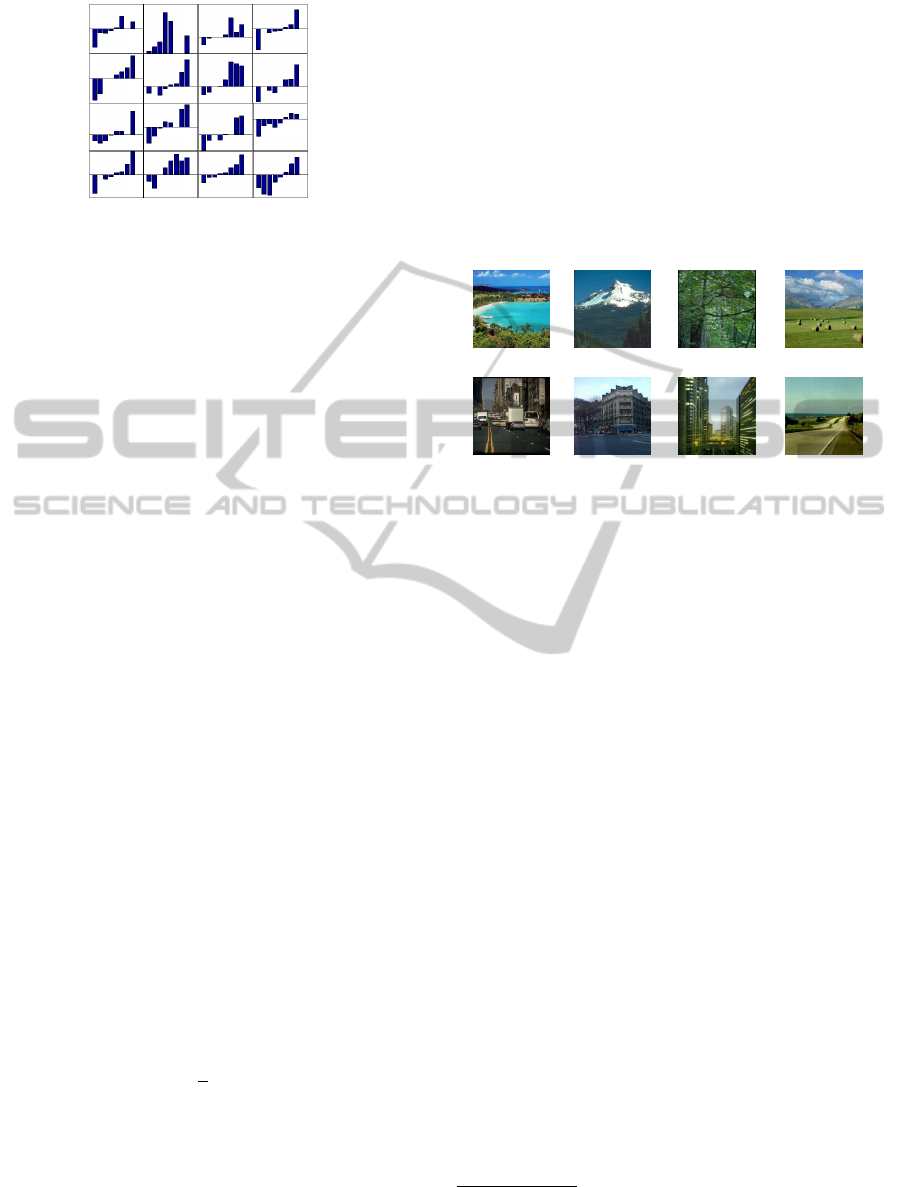
Figure 2: A local patch of 16× 16 pixels is divided into 16
sub-regions. The quantified firing rate values are presented
in each sub-block in the form of an 8-bin histogram.
corresponding to the local feature associated with the
patch.
Note that function (1) is a bounded. To build the
sub-region histograms, we quantify the firing rates ac-
cording to the local rate interval for each patch. This
can be seen as an invariance to changes of luminosity.
A feature will not depend on the probability of a firing
rate compared to the whole image but compared to its
spatial neighbors.
2.4 Global Descriptors and
Classification Task
In the previous section, we have defined dense BiF for
local image description. Those features are sparse.
To deal with classification, we grouped those fea-
tures into Bags-of-Features (Lazebnik et al., 2006).
To this end, we built a dictionary of visual words
from the BiFs extracted in a set of training images
using k-means clustering. Then, for each image, we
formed the Bags-of-bio-inspired Features using hard
histogram assigment.
For classification task, we used the standard ma-
jority vote among the k-nearest neighbors (k-NN).
Namely, a new image is classified by assigning to it
the label present in majority among the labels of its
k-nearest neighbors of the training set in the Bag-of-
bio-inspired Feature space. Let q be the query image,
Cn the number of classes and y
ic
an integer equal to 1
if the image i belongs to the class c ∈ [1,Cn], and zero
otherwise. The classification score h
c
(q) of the im-
age q for the class c is defined as the following k-NN
voting rule:
h
c
(q) =
1
k
∑
j∼
k
q
y
jc
(2)
where j ∼
k
q denotes the j
th
nearest neighbor of q.
The annotation affected to the query is
Y(q) = arg max
c=1..Cn
(h
c
(q))
3 EXPERIMENTS
We tested our approach on the outdoor natural scenes
database
2
proposed in (Oliva and Torralba, 2001). It
contains 2688 annotated images classified into the 8
classes (see Figure 3): coast, mountain, forest, open
country, street, inside city, tall buildings and high-
ways. Let us note that this database is complex
since some images can objectively be assigned to two
classes (for example, street and inside city, or coast
and mountain).
coast mountain forest open country
street inside city tall buildings highways
Figure 3: Examples of natural scenes images from the out-
door database of Torralba (Oliva and Torralba, 2001).
We evaluated the results of classification using the
mean Average Precision (mAP) value (average of the
diagonal values of the confusion matrix).
Dense BiF features were compared to the dense
SIFT features obtained with the VlFeat toolbox
3
(Vedaldi and Fulkerson, 2008) and the dense SIFT
from the LabelMe toolbox
4
(Russell et al., 2008). For
both BiF and SIFT, we formed Bags-of-Features with
which we proceeded with classification.
3.1 Settings
Some parameters have to be set for the extraction of
BiFs. Local dense features are computed over a grid
of points spaced by 10 pixels both horizontally and
vertically. The number of scales used for BiF extrac-
tion is set to 4: this value was chosen empirically.
We should indicate that local features were L2 nor-
malized. Those features were finally transformed into
global descriptors using 1000 visual words to form
L1 normalized Bags-of-Features. Since we are deal-
ing with L1 normalized histogram representations, the
intersection of histograms appears to be a suitable dis-
tance to use in the k-NN frameworkto compare global
descriptors.
For the classification procedure, we need two sep-
arate datasets: the first one for training and the second
2
http://people.csail.mit.edu/torralba/code/spatialenvelope/
3
http://www.vlfeat.org/about.html
4
http://labelme.csail.mit.edu/LabelMeToolbox/index.html
BIO-INSPIRED BAGS-OF-FEATURES FOR IMAGE CLASSIFICATION
279
for testing. We divided the database in a random way,
and we chose 50% of the images to form the training
set and the rest for the testing set.
Experiments reported in the next section are ob-
tained using the k-NN voting rule. We evaluated the
classification using the whole training set images as
k-NN classifiers (or prototypes). And we selected the
value k = 10 for the number of nearest neighbors used
in the classification rule (2). All results were obtained
by cross validations over 10 rounds of test.
3.2 Classification Results
In this section, we give primary classification results
obtained using Bags-of-Features based on BiF and
those based on SIFT from the VlFeat and the La-
belMe toolboxes. Table 1 summarizes the classifica-
tion mAPs. We consider that those results are accu-
rate and promising since we get better performance
than the LabelMe algorithm for dense SIFT.
Table 1: Classification rates for BiF, SIFT of VlFeat toolbox
and SIFT of LabelMe toolbox.
BiF SIFT from VlFeat SIFT from LabelMe
76.72% 77.76% 75.51%
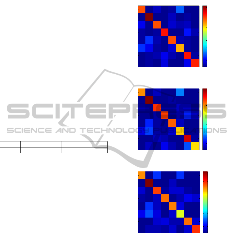
For more details on the classification rates, we
present the confusion matrices in Figure 4, Figure 5
and Figure 6. The coefficient (i, j) of a confusion
matrix corresponds to the classification rate of the i
th
class in the j
th
one. Thus, the diagonal of the ma-
trix matches the rate of correct classifications for each
class.
Confusion matrices presented as classification
maps in Figure 4, Figure 5 and Figure 6 are consistent.
We can note, for example, that both BiF and SIFT de-
scriptors best classify forest images in this database.
This tends to show that our bio-inspired features can
compete with the SIFT.
Although our novel descriptor is relatively simple
and less complex than SIFT (since it deals with lo-
cal contrast intensities), the BiF descriptor seems to
perform similarly to the more mature SIFT descrip-
tor. We think that our approach should be less ex-
pensive in computational time. Although, we did not
evaluate this cost here since the two compared meth-
ods are implemented in different platforms and with
different persons. But, we can argue this conclusion
comparing the main operations in each of them. The
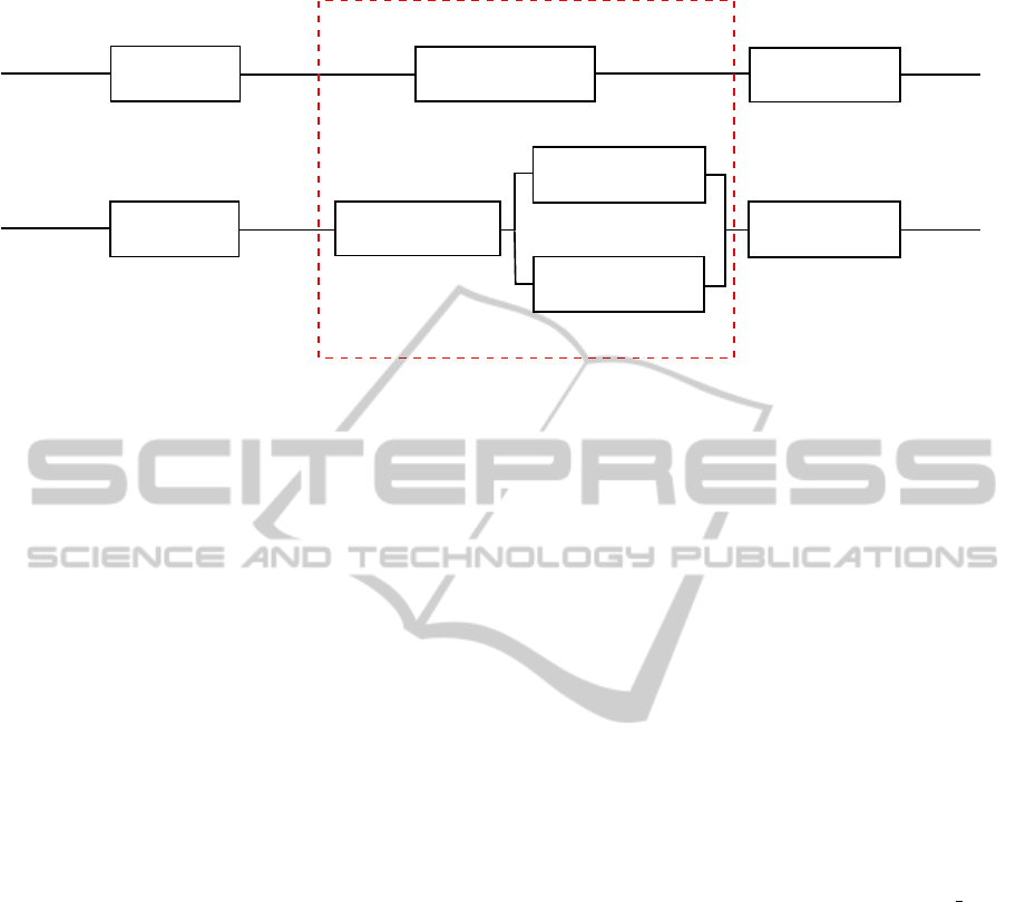
Figure 7, illustrates those operations: both of BiF and
SIFT need smoothing the image at first, and quanti-
fying data to build histograms for final descriptors at
the end. The diffrence is that for BiF, we only need
to compute a simple non-linear function 1 to get the
73.33
92.68
73.07
78.57
73.26
64.39
78.76
77.52
coast
forest
highway
inside city
mountain
open country
street
tall building
0
10
20
30
40
50
60
70
80
90
Figure 4: Confusion matrix for classification test with BiF
descriptors.
70
96.34
79.23
77.27
74.86
63.41
87.67
61.79
coast
forest
highway
inside city
mountain
open country
street
tall building
0
10
20
30
40
50
60
70
80
90
Figure 5: Confusion matrix for classification test with SIFT
descriptors of VlFeat toolbox.
coast
forest
highway
inside city
mountain
open country
street
tall building
10
20
30
40
50
60
70
80
90
69.44
71.91
70.05
72.07
76.92
95.12
77.52
56.09
Figure 6: Confusion matrix for classification test with SIFT
descriptors of LabelMe toolbox.
data to be quantified. When for SIFT, we should com-
pute the gradient using derivatives, then its magnitude
(norm) and its angle (orientation).
We should note that results presented bellow are
elementary and that our approach is still in progress.
This makes this new approach promising for future
works including further optimizations in term of clas-
sification results and computation time.
KDIR 2011 - International Conference on Knowledge Discovery and Information Retrieval
280
Smoothing Compute firing rate
Build histograms
Input image
Contrast
Rate
Descriptors
Smoothing
Compute gradient
Build histograms
Input image
Gaussian
Descriptors
scale space
Compute gradient
Compute gradient
norm
orientation
Figure 7: Main operations to extract BiF descriptors (on top) and SIFT ones (at the bottom). Major differences are steps
within the dashed box.
REFERENCES
Bel Haj Ali, W., Piro, P., Debreuve, E., and Barlaud, M.
(2010). From descriptor to boosting: Optimizing the
k-nn classification rule. In Content-Based Multime-
dia Indexing (CBMI), 2010 International Workshop
on, pages 1–5.
Cortes, C. and Vapnik, V. (1995). Support-vector net-
works. Machine Learning, 20:273–297. 10.1007/
BF00994018.
Delorme, A., Gautrais, J., van Rullen, R., and Thorpe, S.
(1999). Spikenet: A simulator for modeling large net-
works of integrate and fire neurons. Neurocomputing,
26-27:989–996.
Denoeux, T. (1995). A k-nearest neighbor classification rule
based on dempster-shafer theory. Systems, Man and
Cybernetics, IEEE Transactions on, 25(5):804–813.
Escobar, M.-J., Masson, G., Vieville, T., and Kornprobst,
P. (2009). Action recognition using a bio-inspired
feedforward spiking network. International Journal of
Computer Vision, 82:284–301. 10.1007/s11263-008-
0201-1.
Field, D. J. (1994). What is the goal of sensory coding?
Neural Computation, 6(4):559–601.
Freund, Y. and Schapire, R. E. (1995). A decision-theoretic
generalization of on-line learning and an application
to boosting.
Lazebnik, S., Schmid, C., and Ponce, J. (2006). Beyond
bags of features: spatial pyramid matching for recog-
nizing natural scene categories. In IEEE Conference
on Computer Vision and Pattern Recognition, New
York (NY), USA.
Lowe, D. G. (1999). Object recognition from local scale-
invariant features. Computer Vision, IEEE Interna-
tional Conference on, 2:1150.
Oliva, A. and Torralba, A. (2001). Modeling the shape
of the scene: A holistic representation of the spatial
envelope. International Journal of Computer Vision,
42:145–175. 10.1023/A:1011139631724.
Piro, P., Nock, R., Nielsen, F., and Barlaud, M. (2010).
Boosting k-nn for categorization of natural scenes.
ArXiv e-prints.
Rodieck, R. (1965). Quantitative analysis of cat retinal gan-
glion cell response to visual stimuli. Vision Research,
5(12):583–601.
Russell, B., Torralba, A., Murphy, K., and Freeman, W.
(2008). Labelme: A database and web-based tool for
image annotation. International Journal of Computer
Vision, 77:157–173. 10.1007/s11263-007-0090-8.
Schapire, R. E. and Singer, Y. (1999). Improved boosting al-
gorithms using confidence-rated predictions. Machine
Learning, 37:297–336. 10.1023/A:1007614523901.
Sivic, J. and Zisserman, A. (2006). Video google: Effi-
cient visual search of videos. In Ponce, J., Hebert,
M., Schmid, C., and Zisserman, A., editors, Toward
Category-Level Object Recognition, volume 4170 of
Lecture Notes in Computer Science, pages 127–144.
Springer Berlin / Heidelberg. 10.1007/11957959 7.
Thorpe, S. and Gautrais, J. (1998). Rank order coding. In
Proceedings of the sixth annual conference on Com-
putational neuroscience : trends in research, 1998:
trends in research, 1998, CNS ’97, pages 113–118,
New York, NY, USA. Plenum Press.
Thorpe, S. J., Guyonneau, R., Guilbaud, N., Allegraud, J.-
M., and VanRullen, R. (2004). Spikenet: real-time vi-
sual processing with one spike per neuron. Neurocom-
puting, 58-60:857–864. Computational Neuroscience:
Trends in Research 2004.
Van Rullen, R. and Thorpe, S. J. (2001). Rate coding versus
temporal order coding: what the retinal ganglion cells
tell the visual cortex. Neural Comput, 13(6):1255–
1283.
Vedaldi, A. and Fulkerson, B. (2008). VLFeat: An open and
portable library of computer vision algorithms. http://
www.vlfeat.org/.
BIO-INSPIRED BAGS-OF-FEATURES FOR IMAGE CLASSIFICATION
281
