
MULTI-SCALE COMMUNITY DETECTION USING STABILITY
AS OPTIMISATION CRITERION IN A GREEDY ALGORITHM
Erwan Le Martelot and Chris Hankin
Imperial College London, Department of Computing, South Kensington Campus, London SW7 2AZ, U.K.
Keywords:
Community detection, Multi-scale, Multi-resolution, Network analysis, Stability, Modularity, Network
partition, Greedy optimisation, Markov process.
Abstract:
Whether biological, social or technical, many real systems are represented as networks whose structure can be
very informative regarding the original system’s organisation. In this respect the field of community detection
has received a lot of attention in the past decade. Most of the approaches rely on the notion of modularity to
assess the quality of a partition and use this measure as an optimisation criterion. Recently stability was intro-
duced as a new partition quality measure encompassing former partition quality measures such as modularity.
The work presented here assesses stability as an optimisation criterion in a greedy approach similar to mod-
ularity optimisation techniques and enables multi-scale analysis using Markov time as resolution parameter.
The method is validated and compared with other popular approaches against synthetic and various real data
networks and the results show that the method enables accurate multi-scale network analysis.
1 INTRODUCTION
In biology, sociology, engineering and beyond, many
systems are represented and studied as graphs, or net-
works (e.g. protein networks, social networks, web).
In the past decade the field of community detection at-
tracted a lot of interest considering community struc-
tures as important features of real-world networks
(Fortunato, 2010). Given a network of any kind,
looking for communities refers to finding groups of
nodes that are more densely connected internally than
with the rest of the network. The concept considers
the inhomogeneity within the connections between
nodes to derive a partitioning of the network. As op-
posed to clustering methods which commonly involve
a given number of clusters, communities are usually
unknown, can be of unequal size and density and of-
ten have hierarchies (Fortunato, 2010). Finding such
partitioning can provide information about the under-
lying structure of a network and its functioning. It can
also be used as a more compact representation of the
network, for instance for visualisations.
Detecting community structure in networks can be
split into two subtasks: how to partition a graph, and
how to measure the quality of a partition. The latter is
commonly done using modularity (Newman and Gir-
van, 2004). Partitioning graphs is an NP-hard task
(Fortunato, 2010) and heuristics based algorithms ha-
ve thus been devised to reduce the complexity while
still providing acceptable solutions. Considering the
size of some real-world networks much effort is put
into finding efficient algorithms able to deal with
larger and larger networks such as modularity op-
timisation methods. However it has been shown
that networks often have several levels of organisa-
tion (Simon, 1962), leading to different partitions for
each level which modularity optimisation alone can-
not handle (Fortunato, 2010). Methods have been pro-
vided to adapt modularity optimisation to multi-scale
(multi-resolution) analysis using a tuning parameter
(Reichardt and Bornholdt, 2006; Arenas et al., 2008).
Yet the search for a partition quality function that ac-
knowledges the multi-resolution nature of networks
with appropriate theoretical foundations has received
less attention. Recently, stability (Delvenne et al.,
2010) was introduced as a new quality measure for
community partitions. Here we investigate its use as
an optimisation criterion for multi-scale analysis. We
show how stability can be used in place of modularity
in modularity optimisation methods and present a new
greedy agglomerative algorithm using stability as op-
timisation function and enabling multi-scale analysis
using Markov time as a resolution parameter.
The next section reviews related work. Then our
method is presented followed by experiments assess-
ing its potential, discussion and conclusion.
216
Le Martelot E. and Hankin C..
MULTI-SCALE COMMUNITY DETECTION USING STABILITY AS OPTIMISATION CRITERION IN A GREEDY ALGORITHM.
DOI: 10.5220/0003655002080217
In Proceedings of the International Conference on Knowledge Discovery and Information Retrieval (KDIR-2011), pages 208-217
ISBN: 978-989-8425-79-9
Copyright
c
2011 SCITEPRESS (Science and Technology Publications, Lda.)

2 BACKGROUND
While several community partition quality measures
have been used (Fortunato, 2010), the most com-
monly found in the literature is modularity (Newman
and Girvan, 2004). Given a partition into c communi-
ties let e be the community matrix of size c × c where
each e
i j
gives the fraction of links going from a com-
munity i to a community j and a
i
=
∑
j
e
i j
the fraction
of links connected to i. (If the graph is undirected,
each e
i j
not on the diagonal should be given half of
the edges connecting communities i and j so that the
number of edges connecting the communities is given
by e
i j
+e
ji
(Newman and Girvan, 2004).) Modularity
Q
M
is the sum of the difference between the fraction
of links within a partition linking to this very parti-
tion minus the expected value of the fraction of links
doing so if edges were randomly placed:
Q
M
=
c
∑
i=1
(e
ii
− a
2
i
) (1)
One advantage of modularity is to impose no con-
straint on the shape of communities as opposed for
instance to the clique percolation method (Palla et al.,
2005) that defines communities as adjacent k-cliques
thus imposing that each node in a community is part
of a k-clique.
Modularity was initially introduced to evaluate
partitions. However its use has broadened from
partition quality measure to optimisation function
and modularity optimisation is now a very common
approach to community detection (Newman, 2004;
Clauset et al., 2004; Newman, 2006; Blondel et al.,
2008). (Recent reviews and comparisons of com-
munity detection methods including modularity op-
timisation methods can be found in (Fortunato, 2010;
Lancichinetti and Fortunato, 2009).) Modularity op-
timisation methods commonly start with each node
placed in a different community and then successively
merge the communities that maximise modularity at
each step. Modularity is thus locally optimised at
each step based on the assumption that a local peak
should indicate a particularly good partition. The first
algorithm of this kind was Newman’s fast algorithm
(Newman, 2004). Here, for each candidate partition
the variation in modularity ∆Q
M
that merging two
communities i and j would yield is computed as
∆Q
M
i j
= 2(e
i j
− a
i
a
j
) (2)
where i and j are the communities merged in the new
candidate partition. Computing only ∆Q
M
minimises
the computations required to evaluate modularity and
leads to the fast greedy algorithm given in Algorithm
1. This algorithm enables the incremental building
Algorithm 1: Greedy algorithm sketch for modularity opti-
misation.
1. Divide in as many clusters as there are nodes.
2. Measure modularity variation ∆Q
M
for each can-
didate partition where a pair of clusters are
merged.
3. Select the network with the highest ∆Q
M
.
4. Go back to step 2.
of a hierarchy where each new partition is the local
optima maximising Q
M
at each step. It was shown
to provide good solutions with respect to the original
Girvan-Newman algorithm that performs accurately
but is computationally highly demanding and is thus
not suitable for large networks (Newman and Girvan,
2004). (Note that accuracy refers in this context to a
high modularity value. Other measures, such as sta-
bility, might rank partitions differently.) Since then
other methods have been devised such as (Clauset
et al., 2004) optimising the former method, another
approach based on the eigenvectors of matrices (New-
man, 2006) or the Louvain method (Blondel et al.,
2008). The last method has shown to outperform in
speed previous greedy modularity optimisation meth-
ods by reducing the number of intermediate steps for
aggregating all the nodes.
These methods all rely on modularity optimisa-
tion. Yet modularity optimisation suffers from sev-
eral issues. One issue is known as the resolution limit
meaning that modularity optimisation methods can
fail to detect small communities or over-partition net-
works (Fortunato and Barth
´
elemy, 2007) thus miss-
ing the most natural partitioning of the network. An-
other issue is that the modularity landscape admits a
large number of structurally different high-modularity
value solutions and lacks a clear global maximum
value (Good et al., 2010). It has also been shown
that random-graphs can have a high modularity value
(Guimer
`
a et al., 2004).
Some biases have been introduced to alter the be-
haviour of the method towards communities of var-
ious sizes (Danon et al., 2006; Reichardt and Born-
holdt, 2006; Arenas et al., 2008). In (Danon et al.,
2006), the authors observed that large communities
are favoured at the expense of smaller ones biasing
the partitioning towards a structure with a few large
clusters which may not be an accurate representation
of the network. They provided a normalised measure
of ∆Q
M
defined as
∆Q
0
M
i j
= max
∆Q
M
i j
a
i
,
∆Q
M
i j
a
j
(3)
MULTI-SCALE COMMUNITY DETECTION USING STABILITY AS OPTIMISATION CRITERION IN A GREEDY
ALGORITHM
217

which aims at treating communities of different sizes
equally. In (Reichardt and Bornholdt, 2006), modu-
larity optimisation is modified by using a scalar pa-
rameter γ in front of the null term (the fraction of
edges connecting vertices of a same community in a
random graph) turning equation (1) into
Q
M
γ
=
∑
i
(e
ii
− γa
2
i
) (4)
where γ can be varied to alter the importance given
to the null term (modularity optimisation is found for
γ = 1). In (Arenas et al., 2008), modularity optimi-
sation is performed on a network where each node’s
strength has been reinforced with self loops. Consid-
ering the adjacency matrix A, modularity optimisation
is performed on A + rI where I is the identity matrix
and r is a scalar. Varying the value of r enables the
detection of communities at various coarseness levels
(modularity optimisation is found for r = 0). With
their resolution parameter, the two latter methods en-
able a multi-scale network analysis.
Significant attention has been given to modular-
ity but little attention has been given to new partition
quality measures. Recently, stability was introduced
in (Delvenne et al., 2010) as a new partition quality
measure unifying some known clustering heuristics
including modularity and using Markov time as an in-
ner resolution parameter. The stability of a graph con-
siders the graph as a Markov chain where each node
represents a state and each edge a possible state tran-
sition. Let n be the number of nodes, m the number
of edges, A the n × n adjacency matrix containing the
weights of all edges (the graph can be weighted or
not), d a size n vector giving for each node its degree
(or strength for a weighted network) and D = diag(d)
the corresponding diagonal matrix. The stability of a
graph considers the graph as a Markov chain where
each node represents a state and each edge a possible
state transition. The chain distribution is given by the
stationary distribution π =
d
2m
. Let also Π be the cor-
responding diagonal matrix Π = diag(π). The transi-
tion between states is given by the n×n stochastic ma-
trix M = D
−1
A. Assuming a community partition, let
H be the indicator matrix of size n × c giving for each
node its community. The clustered auto-covariance
matrix at Markov time t is defined as:
R
t
= H
T
(ΠM
t
− π
T
π)H (5)
Stability at time t noted Q
S
t
is given by the trace of
R
t
and the global stability measure Q
S
considers the
minimum value of the Q
S
t
over time from time 0 to a
given upper bound τ:
Q
S
= min
0≤t≤τ
trace(R
t
) (6)
This model can be extended to deal with real values
of t by using the linear interpolation:
R
t
= (c(t) − t) · R( f (t)) + (t − f (t)) · R(c(t)) (7)
where c(t) returns the smallest integer greater than t
and f (t) returns the greatest integer smaller than t.
This is useful to investigate for instance time values
between 0 and 1. It was indeed shown in (Delvenne
et al., 2010) that the use of Markov time with values
between 0 and 1 enables detecting finer partitions than
those detected at time 1 and above.
Also, this model can be turned into a continuous
time Markov process by using the expression e
(M−I)t
in place of M
t
(where e is the exponential function)
(Delvenne et al., 2010).
Stability has been introduced as a measure to eval-
uate the quality of a partition hierarchy and has been
used to assess the results of various modularity op-
timisation algorithms. Further mathematical founda-
tions have been presented in (Lambiotte et al., 2008;
Lambiotte, 2010). The work presented here investi-
gates stability as an optimisation function with var-
ious practical test cases. It presents and assesses a
greedy algorithm that optimises stability similarly to
modularity optimisation methods and uses stability’s
inner Markov time as a resolution parameter. While
related approaches such as Arenas et al’s and Re-
ichardt et al’s methods also offer a multi-scale anal-
ysis with their respective parameters, these methods
offer a tuneable version of modularity optimisation
by modifying the importance of the null factor or by
adding self-loops to nodes. Such analysis remains
based on a one step random walk analysis of the net-
work with modifications of its structure. Stability op-
timisation enables on the contrary random walks of
variable length defined by the Markov time thus ex-
ploiting thoroughly the actual topology of the net-
work. As communities reflect the organisation of
a network, and hence its connectivity, this approach
seems to be more suitable. The next section presents
the method followed by experiments assessing it and
comparing it to other relevant approaches.
3 METHOD
As discussed in (Delvenne et al., 2010) the measure of
stability and the investigation of stability of a partition
along the Markov time (stability curve) for a partition
can help addressing the partition scale issue and the
optimal community identification. The results from
the authors indeed show with the stability curve that
the clustering varies depending on the time window
during which the Markov time is considered. From
KDIR 2011 - International Conference on Knowledge Discovery and Information Retrieval
218

there, our work uses the Markov time as a resolution
parameter in an optimisation context where stability
is used as the optimisation criterion.
Considering the Markov chain model, it has been
shown in (Delvenne et al., 2010) that stability at time
1 is modularity. From equation (5) it can also be
derived that stability at time t is the modularity of
a graph whose adjacency matrix is A
t
= DM
t
(or
A
t
= De
(M−I)t
for the continuous time model).
Considering stability at time t as the modularity
of a graph given by the adjacency matrix A
t
allows
us to apply the work done on modularity optimisa-
tion to stability. Stability optimisation then becomes a
broader measure where modularity is the special case
t = 1 in the Markov chain. Using the modularity no-
tation from equation (1), stability at time t can be de-
fined as:
Q
S
t
=
∑
i
(e
t
ii
− a
2
i
) (8)
where e
t
is the community matrix for Markov time t
computed from A
t
.
Modularity optimisation is based on computing
the change in modularity between an initial partition
and a new partition where two clusters have been
merged. The change in modularity when merging
communities i and j is given by equation (2) and sim-
ilarly the change in stability at time t is
∆Q
S
t
i j
= 2(e
t
i j
− a
i
a
j
) (9)
Following equation (6) the new Q
S
value Q
0
S
is:
Q
0
S
= min
0≤t≤τ
(Q
S
t
+ ∆Q
S
t
) (10)
At each clustering step, the partition with the best Q
0
S
value is kept and Q
S
is then updated as Q
S
= Q
0
S
. For
computational reasons the time needs to be sampled
between 0 and τ. Markov time can be sampled lin-
early or following a log scale. The latter is usually
more efficient for large time intervals.
The matrices e
t
are computed in the initialisation
step of the algorithm and then updated by succes-
sively merging the lines and columns corresponding
to the merged communities. This leads to the greedy
stability optimisation (GSO) algorithm given in Algo-
rithm 2, based on the principle of Algorithm 1.
Depending on the Markov time boundaries the
partitions will vary as the larger the time window, the
longer a partition must keep a high stability value to
get a high overall stability value, as defined in equa-
tion (6). The Markov time thus acts as a resolution
parameter.
Compared to Newman’s fast algorithm the addi-
tional cost of stability computation and memory re-
quirement is proportional to the number of times con-
sidered in the Markov time window. For each time
t considered in the computation, a matrix e
t
must be
computed and kept in memory. Let n be the number
of nodes in a network, m the number of edges and s
the number of time steps required for stability com-
putation. The number of merge operations needed to
terminate are n − 1. Each merging operation requires
to iterate through all edges, hence m times, and for
each edge to compute the stability variation s times.
The computation of each ∆Q can be performed in
constant time. In a non optimised implementation the
merging of communities i and j can be performed in n
steps, hence the complexity of the algorithm would be
O(n(m.s + n)). However the merging of communities
i and j really consists in adding the edges of commu-
nity j to i and then deleting j. To do so there is one
operation per edge. The size of a cluster at iteration
i is given by cs(i) =
n
n−i
. and therefore the average
cluster size over all iterations is
¯cs =
1
n
·
n
∑
i=1
cs(i) =
n
∑
i=1
1
i
≈ ln(n) + γ (11)
with γ the Euler-Mascheroni constant. As the number
of edges is bounded by the number of nodes squared,
the algorithm can be implemented with the complex-
ity O (n(m.s + ln
2
(n))) provided the appropriate data
structures are used to exploit this, as discussed in
(Clauset et al., 2004). Considering that s should be
low, the complexity is O(n(m + ln
2
(n))).
Also a large time window does not imply many
time values. The speed-accuracy trade-off comes
from the number of steps s within the boundaries,
whatever the boundaries. While the full mathematical
definition of stability considers all Markov times in a
given interval, all Markov times may not be crucial
to a good (or even exact) approximation of stability.
The fastest way to approximate stability is to compute
it with only one time value. As stability tends to de-
crease as the Markov time increases, we are seeking
when the following approximation can be made:
Q
S
= min
0≤t≤τ
trace(R
t
) ≈ trace(R
τ
) (12)
The need for considering consecutive time values in
the computation of stability addresses an issue en-
countered within random walks. Considering for in-
stance a graph with three nodes a, b and c with an
edge between nodes a and b and between nodes b and
c. Using a Markov time of 2 only (i.e. a random walk
of 2 steps with no consideration of the first step) start-
ing from a there would be no transition between a and
b as after one step from a the random walker would
be in b and then it could only go back to a or walk
to c. However, the more densely connected the clus-
ters, the less likely this situation is to happen as many
paths can be borrowed to reach each node. This time
MULTI-SCALE COMMUNITY DETECTION USING STABILITY AS OPTIMISATION CRITERION IN A GREEDY
ALGORITHM
219

optimisation is assessed with the rest of the method in
the next section.
4 EXPERIMENTS & RESULTS
To assess our method we use various known networks
made of real or synthetic data that have been used in
related work and are publicly available. For compari-
son, other relevant methods are tested along with our
method: Newman’s fast algorithm (Newman, 2004),
Danon et al’s method (Danon et al., 2006), the Lou-
vain method (Blondel et al., 2008), Reichardt et al’s
method (Reichardt and Bornholdt, 2006), and Arenas
et al’s method (Arenas et al., 2008). Both Reichardt
et al’s and Arenas et al’s methods use a resolution pa-
rameter that enables multi-scale community detection
based on this parameter. The Louvain method also
returns a succession of partition (not tuneable). The
other two methods are not multi-scale and hence only
return one partition.
The community detection algorithms were imple-
mented in Matlab
1
except for the code of the Lou-
vain method downloaded from the authors website
2
(we used their hybrid C++ Matlab implementation).
All experiments were run using Matlab R2010b un-
der MacOS X on an iMac 3.06GHz Intel Core i3.
4.1 Networks
The networks considered are two synthetic and four
real-world data networks
3
that have been used as
benchmarks in the literature to assess community de-
tection algorithms. The networks have been chosen
for their respective properties (e.g. multi-scale, scale-
free) and popularity that enable an assessment of
our method and comparisons with other approaches.
While selecting very large networks can demonstrate
speed efficiency, the results are commonly ranked us-
ing modularity which as previously discussed is not
suitable for this work. We therefore deemed appro-
priate to use here networks of smaller size with some
knowledge of their structure or content used for the
evaluation of the results, similarly to what has been
done in related work (Reichardt and Bornholdt, 2006;
Arenas et al., 2008).
1
The code developed for this work is available on re-
quest. More also at http://www.elemartelot.org.
2
http://sites.google.com/site/findcommunities/
3
Available from http://www-
personal.umich.edu/ mejn/netdata/
4.1.1 Synthetic Datasets
Ravasz et al’s Scale-free Hierarchical Network.
This network was presented in (Ravasz and Barab
´
asi,
2003) and defines a hierarchical network of 125 nodes
as shown in Figure 1(a). The network is built itera-
tively from a small cluster of 5 densely linked nodes.
A node at the centre of a square is connected to 4 oth-
ers at the corners of the square themselves also con-
nected to their neighbours. Then 4 replicas of this
cluster are generated and placed around the first one,
producing a 25 nodes network. The centre of the cen-
tral cluster is linked to the corner nodes of the other
clusters. This process is repeated again to produce the
125 nodes network. The structure can be seen as 25
clusters of 5 nodes or 5 clusters of 25 nodes.
Arenas et al’s Homogeneous in Degree Network.
This network taken from (Arenas et al., 2006) and
named H13-4 is a two hierarchy levels network of 256
nodes organised as follow. 13 edges are distributed
between the nodes of each of the 16 communities
of the first level (internal community) formed of 16
nodes each. 4 edges are distributed between nodes of
each of the 4 communities of the second level (exter-
nal community) formed of 64 nodes each. 1 edge per
node links it with any community of the rest of the
network. The network is presented in Figure 1(b).
(a) Ravasz 125 nodes. (b) H13-4.
Figure 1: (a) Hierarchical scale free network generated in 3
steps producing 125 nodes at step 3 (Ravasz and Barab
´
asi,
2003). (b) Network presented in (Arenas et al., 2006) made
of 256 nodes organised in two hierarchical levels with 16
communities of 16 nodes for the first level and 4 communi-
ties of 64 nodes for the second level.
4.1.2 Real-world Datasets
Zachary’s Karate Club. This network is a social
network of friendships between 34 members of a
karate club at a US university in 1970 (Zachary,
1977). Following a dispute the network was divided
into 2 groups between the club’s administrator and the
club’s instructor. The dispute ended in the instructor
creating his own club and taking about half of the ini-
tial club with him. The network can hence be divided
into 2 main communities. A division into 4 communi-
ties has also been acknowledged (Medus et al., 2005).
KDIR 2011 - International Conference on Knowledge Discovery and Information Retrieval
220

Algorithm 2: Greedy stability optimisation (GSO) algorithm taking in input an adjacency matrix and a Markov time window,
and returning a partition and its stability value.
Divide in as many communities as there are nodes
Set this partition as current partition C
cur
and as best known partition C
Set its stability value as best known stability Q
Set its stability vector (stability values at each Markov time) as current stability vector QV
Compute initial community matrix e
Compute initial community matrices at Markov times e
t
while 2 communities at least are left in current partition: length(e) > 1 do
Initialise best loop stability Q
loop
← −∞
for all pair of communities with edges linking them: e
i j
> 0 do
for all times t in time window do
Compute dQV (t) ← ∆Q
S
t
end for
Compute partition stability vector: QV
tmp
← QV + dQV
Compute partition stability value by taking its minimum value: Q
tmp
← min(QV
tmp
)
if current stability is the best of the loop: Q
tmp
> Q
loop
then
Q
loop
← Q
tmp
QV
loop
← QV
tmp
Keep in memory best pair of communities (i, j)
end if
end for
Compute C
cur
by merging the communities i and j
Update all community matrices e and e
t
by merging rows i and j and columns i and j
Set current stability vector to best loop stability vector: QV ← QV
loop
if best loop stability higher than best known stability: Q
loop
> Q then
Q ← Q
loop
C ← C
cur
end if
end while
return best found partition C and its stability Q
Lusseau et al’s Dolphins Social Network. This
network is an undirected social network resulting
from observations of a community of 62 bottle-nose
dolphins over a period of 7 years (Lusseau et al.,
2003). Nodes represent dolphins and edges represent
frequent associations between dolphin pairs occurring
more often than expected by chance. Analysis of the
data revealed 2 main groups and a further division can
be made into 4 groups (Lusseau and Newman, 2004).
American College Football Dataset. This dataset
contains the network of American football games
(Girvan and Newman, 2002). The 115 nodes repre-
sent teams and the edges represent games between
2 teams. The teams are divided into 12 groups con-
taining around 8-12 teams each and games are more
frequent between members of the same group. Also
teams that are geographically close but belong to dif-
ferent groups are more likely to play one another than
teams separated by a large distance. Therefore in this
dataset the groups can be considered as known com-
munities.
Les Mis
´
erables. This dataset taken from (Knuth,
1993) represents the co-appearance of 77 characters
in Victor Hugo’s novel Les Mis
´
erables. Two nodes
share an edge if the corresponding characters appear
in a same chapter of the book. The values on the edges
are the number of such co-appearances.
4.2 Results
The networks are analysed by the 5 aforementioned
community detection methods and our stability opti-
misation algorithm for which both discrete and con-
tinuous Markov time versions are used. Also two time
window setups are considered to investigate the ap-
proximation from equation (12): one that considers a
time window [0, τ] and another that considers only τ.
Table 1 provides the results of the community de-
tection methods that have no resolution parameter.
The results show that these methods do not necessar-
ily find the most meaningful partitions and that differ-
ent methods can identify different partitions. Yet this
does not imply that an unexpected result is meaning-
less. For example in Ravasz et al’s network, the cen-
tral node of the central community has many more
connections than the other nodes and more connec-
tions outside its community than inside. Therefore
this node can be seen as a community on its own.
Figure 2 plots the results of the tuneable meth-
MULTI-SCALE COMMUNITY DETECTION USING STABILITY AS OPTIMISATION CRITERION IN A GREEDY
ALGORITHM
221
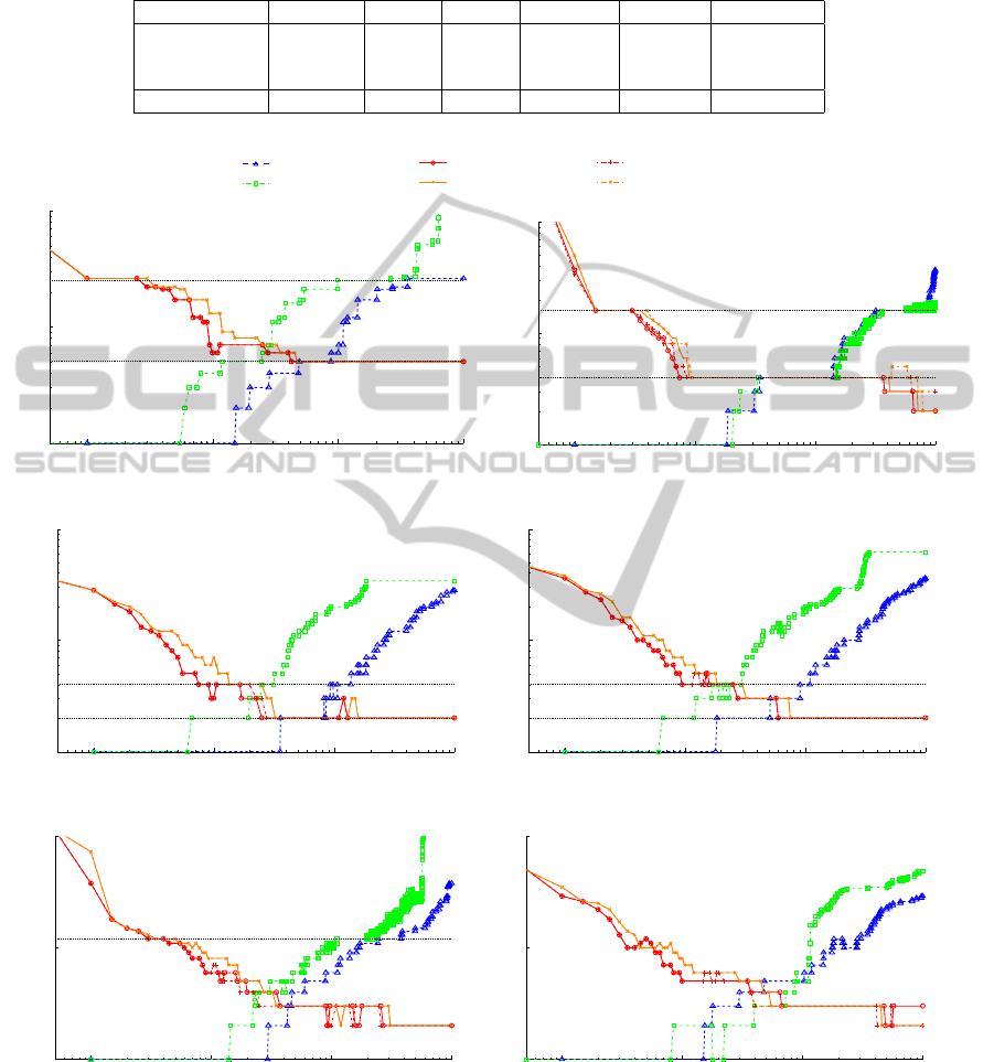
Table 1: Number of detected communities by fast Newman, Louvain and Danon et al’s methods on the presented networks.
The identified division(s) known for these networks are also indicated (’-’ indicates that there is no clear a priori knowledge).
The Louvain method returns a hierarchy of partitions, given in order.
Algorithm Ravasz H13-4 Karate Dolphins Football Miserables
Fast Newman 6 4 3 4 6 5
Danon 6 4 4 4 6 6
Louvain 30, 10, 6 12, 4 6, 4 10, 5 12, 10 9, 6
Identified 5, 25 4, 16 2, 4 2, 4 12 -
10
−1
10
0
10
1
10
2
10
0
10
1
10
2
Parameter
Number of Communities
(a) Ravasz et al’s network.
10
−1
10
0
10
1
10
2
10
0
10
1
10
2
Parameter
Number of Communities
(b) Hierarchical 13-4 network.
10
−1
10
0
10
1
10
2
10
0
10
1
10
2
Parameter
Number of Communities
(c) Karate club network.
10
−1
10
0
10
1
10
2
10
0
10
1
10
2
Parameter
Number of Communities
(d) Dolphins social network.
10
−1
10
0
10
1
10
2
10
0
10
1
10
2
Parameter
Number of Communities
(e) American football network.
10
−1
10
0
10
1
10
2
10
0
10
1
10
2
Parameter
Number of Communities
(f) Les Mis
´
erables characters network.
Figure 2: Number of partitions returned by Reichardt et al’s, Arenas et al’s and our stability optimisation methods. The x-axis
represents 10γ for Reichardt et al’s method, r − r
0
for Arenas et al’s and t for ours. The setup using a time window is noted
[0,t] while the setup using only one time value is noted t. The time discrete Markov model (Markov chain) is noted (Dis) and
the time continuous Markov model is noted (Con). The dotted horizontal lines indicate known partitions size: (a) 5 and 25,
(b) 4 and 16, (c) 2 and 4, (d) 2 and 4, (e) 12.
KDIR 2011 - International Conference on Knowledge Discovery and Information Retrieval
222

ods along their respective parameter values. For Re-
ichardt et al’s algorithm, the x-axis represents 10γ.
For Arenas et al’s the x-axis represents r − r
0
where
r
0
= −
m
n
with m the number of edges and n the num-
ber of nodes. (See (Arenas et al., 2008) for details.
The authors use the lower bound r
asymp
= −
2m
n
but
here we found that values of r below r
0
were irrele-
vant.) The value of r
0
is calculated for each network.
For our algorithm, the x-axis represents the Markov
time t. For the time window setup the sampling is
done from time 0 to 100 with a step of 0.05 between
within [0, 2], a step of 0.25 within [2, 10] and a step
of 1 afterwards. The steps between successive values
of the parameter are 0.05 for Arenas and
0.05
10
= 0.005
for Reichardt et al’s (as the x-axis represents 10γ).
Considering only stability optimisation we can ob-
serve that the two Markov processes behave in a very
similar way. We can also observe that the difference
between the runs considering the time window and
those considering only its upper bound is minimal.
The curves are similar or overlapping thus suggesting
that the approximation from equation (12) holds.
From Figure 2 it can be observed that the be-
haviour of our method is opposite to those of the two
other tuneable methods. At low values of t partitions
are small (at t = 0 our method finds as many parti-
tions as there are nodes). Then as t increases, parti-
tions tend to become larger. Conversely, the two other
methods start by partitioning in large clusters when
their parameter is minimal. Then they find finer par-
titions as their parameter increases. As the discrete
and continuous time versions of our algorithm have a
very similar behaviour, and as the time optimised se-
tups almost overlap with the full time interval setups,
we will only comment on the discrete time version.
Considering Figure 2(a) for instance, after t = 4,
the result of our algorithm remains stable on 5 clus-
ters that represent the most stable partition. A parti-
tion in 6 elements can also be found and corresponds
to the 5 large communities with the centre of the cen-
tral community in a separate community. Also, when
t ∈ [0.1, 0.2] the algorithm finds a partition in 26 com-
munities (25 small communities plus central node on
its own). Arenas et al’s method detects the 5 commu-
nities around about r − r
0
∈ [1.5, 2.5]. Then it grows
to stabilise on 25 communities around r − r
0
∈ [9, 25]
and then goes up to 26 communities and more. Re-
ichardt et al’s stabilises around 5 communities around
γ = [0.5, 0.9] and around 26 communities around γ =
3.6 and onwards. Looking at the stability optimisa-
tion and Reichardt et al’s method compared to Are-
nas et al’s method, the two former tend to stabilise at
intermediate partitions of a size 1 larger than those
detected by the latter. By using the resistance pa-
rameter r, Arenas et al’s method alters the impact of
edge weights across the network. In this instance this
blends the central node into the small central com-
munity. However when considering the partition in
25 communities, this central node has 4 connections
with all communities, including its own. By adding
it to any community, this community would gain 4
edges pointing inside and 80 pointing outside. There-
fore it is ambiguous whether this node should belong
to the small central community or any of the others.
This is handled in our method by keeping this node in
a separate community until it is clear that it belongs to
the central community of the 5 communities partition
(it then shares 20 edges inside its own community and
16 edges with each of the 4 others).
On Figure 2(b), the intended partitions in 16 and
then 4 communities are clearly detected. As expected
the most stable partition is the partition in 4 communi-
ties, as indicated by the stability optimisation methods
with the long stretch of time settling on this partition
compared to the shorter plateau for 16 communities.
Considering Figure 2(c), our algorithm quickly
settles on the 2 expected partitions, found by Arenas
et al’s for about r − r
0
∈ [0.7, 2] and by Reichardt et
al’s for about γ ∈ [0.4, 0.8]. It also consistently set-
tles beforehand on the partition in 4 communities, re-
vealing the relevance of this partition, as suggested by
other analysis (Medus et al., 2005).
Regarding Figure 2(d), our algorithm settles on 2
partitions, as expected from the results (Lusseau and
Newman, 2004) that analysed the dataset using mod-
ularity. Arenas et al’s solution for r − r
0
∈ [0.7, 1.2]
and Reichardt et al’s solution for γ ∈ [0.2, 0.5] cor-
responds to the partition of (Lusseau and Newman,
2004). Our algorithm also stops over on 4 partitions
for t ∈ [0.5, 3[ \1.5 which is another relevant division
size of the network (Lusseau and Newman, 2004).
On Figure 2(e) we can observe several scales of
relevance. Based on the knowledge of the teams dis-
tribution, a community of size 12 is expected. Such
partition is detected at an early time (t = 0.3) with
our method and is the first plateau. A normalised mu-
tual information value of 0.919 compared with the
12 known groups can be found by our method on
this plateau. Most of the nodes are therefore placed
into the right communities. Regarding the remaining
nodes, (Khadivi et al., 2011) explains that some nodes
do not fit in the expected classification. Therefore
other divisions can also be of relevance. While sta-
bility settles on a few plateaus the two other methods
tend to detect shortly many intermediate partitions.
As the time grows communities also grow bigger and
get more stable. A partition into 3 communities is
consistently identified followed by a partition with 2
MULTI-SCALE COMMUNITY DETECTION USING STABILITY AS OPTIMISATION CRITERION IN A GREEDY
ALGORITHM
223

communities. Analysing the former we find that it re-
flects the geographical locations of the teams, reflect-
ing the fact that teams located geographically closer
are more likely to play one another. This partition sep-
arates the country roughly into West, South-east and
North-east. Then the partition with 2 communities di-
vides the country into West and East. Therefore the
successive stable partitions reflect the organisation of
the teams, first locally with the 12 communities par-
tition and then nationally with the partitions in 3 and
2 communities (other partitions in between may also
reflect smaller geographical divisions). Another anal-
ysis could consider the large and stable communities
(e.g. of size 2 or 3) and sub-partition them to analyse
the games distribution at a smaller geographical scale.
Analysing the network of the characters from Les
Mis
´
erables several divisions appear. Considering sta-
bility optimisation 2 main partitions appear, as shown
on Figure 2(f), while the other methods detect more
partitions on short intervals. The first one consistently
identified by our method contains 5 communities and
the second one contains 3 communities. In the parti-
tion into 5 communities the first is a central commu-
nity containing most of the main plot characters such
as Valjean, Javert, Cosette, Marius or the Thenardier.
The second community relates to the story of Fantine,
the third one relates to Mgr Myriel, the fourth one
relates to Valjean’s story as a prisoner and contains
other convicts. The fifth one relates to Gavroche, an-
other main character. Considering the partition in 3
communities, the central community is merged with
the fourth community (convicts, judge, etc) and the
third community. The community mainly represents
characters connected to Valjean at a moment of his
story. The second community remains as well as the
fifth one with Marius now part of it.
These results highlight the fact that different meth-
ods provide different approaches and solutions to the
problem of community partitions. Consistent or sta-
ble partitions are used to identify relevant divisions
in a network. Considering the three tuneable meth-
ods the results show that stability optimisation tends
to stabilise on fewer partitions and often more con-
sistently than the other two methods. This is use-
ful to identify most relevant partitions and hence in-
form about networks structure in the absence of a pri-
ori knowledge. To better detect stable partitions the
normalised mutual information (NMI) (Fred and Jain,
2003) between successive partitions (e.g. found at
times t and t + dt) was also sometimes used. A per-
sistent high NMI value confirms that successive parti-
tions of same size are indeed the same or similar, thus
ruling out the possibility of having different partitions
that happen to have the same number of communities.
5 CONCLUSIONS
This work investigated stability as an optimisation
criterion for a greedy approach similar to the one
used in (Newman, 2004; Danon et al., 2006; Re-
ichardt and Bornholdt, 2006; Arenas et al., 2008).
The results showed that our method enables accurate
multi-scale analysis and tackles the problem differ-
ently than other methods by finding stable partitions
over a Markov time which is part of the definition of
stability. The method was tested against various net-
works and compared to five relevant community de-
tection algorithms. Stability optimisation can be seen
as an extension of modularity optimisation that does
not alter the graph (like Arenas et al’s) or the impor-
tance of the null factor (like Reichardt et al’s) but in-
stead exploits the graph by interpreting it as a Markov
process. By analysing it over different time scales it
explores the graph thoroughly by considering paths
of various lengths between nodes where each consid-
ered Markov time defines a path length. This analysis
can be performed without complexity increase com-
pared to modularity optimisation methods such as fast
Newman’s algorithm. Two Markov processes have
been tested for our method, one based on a Markov
chain model of a network and the other one extending
this model to a continuous time Markov process. Ex-
periments showed that both models behave similarly
considering the cases studied in this work. They also
showed that stability can be optimised with almost no
loss of accuracy by only using the upper bound of a
Markov time interval, as opposed to the whole inter-
val suggested by the mathematical definition of stabil-
ity. This heuristic provides a significant gain in speed.
The results showed that multiple levels of organ-
isations are clearly identified when optimising sta-
bility over time. Stability optimisation tends to set-
tle for longer on fewer partitions than other related
approaches considered here, thus highlighting better
partitions of relevance. Stability optimisation also
converges towards large and stable clusters. This be-
haviour also differs from those of other approaches
and in the absence of a priori knowledge our method
has therefore the advantage of leading to stable and
relevant communities from where a deeper analysis
could be performed in each community subgraph.
The complexity of our method with the time-
optimised heuristic is in O(n(m + ln
2
(n))) which
compares to similar approaches using modularity and
scaling to large networks. Therefore our method
should scale up very well to large networks.
Further work will consider a randomised algo-
rithm similarly to the randomised modularity optimi-
sation algorithm presented in (Ovelg
¨
onne et al., 2010)
KDIR 2011 - International Conference on Knowledge Discovery and Information Retrieval
224

that would reduce the complexity to O (n · ln
2
(n)).
Another possible optimisation is a multi-step ap-
proach as presented in (Schuetz and Caflisch, 2008)
for modularity optimisation. This work can also be
applied to detecting overlapping communities by us-
ing the line graph of the initial graph as in (Pereira-
Leal et al., 2004), thus working on link communities
(Ahn et al., 2010). Further work could also consider
a self-tuneable algorithm that returns the most stable
partition(s). Another algorithm could then provide a
stable hierarchy by repeatedly subdividing the stable
partitions found at each hierarchical level.
REFERENCES
Ahn, Y.-Y., Bagrow, J. P., and Lehmann, S. (2010). Link
communities reveal multiscale complexity in net-
works. Nature, 466:761–764.
Arenas, A., D
´
ıaz-Guilera, A., and P
´
erez-Vicente, C. J.
(2006). Synchronization reveals topological scales in
complex networks. Physical Review Letters.
Arenas, A., Fernandez, A., and Gomez, S. (2008). Anal-
ysis of the structure of complex networks at different
resolution levels. New Journal of Physics, 10:053039.
Blondel, V. D., Guillaume, J.-L., Lambiotte, R., and Lefeb-
vre, E. (2008). Fast unfolding of communities in large
networks. Journal of Statistical Mechanics: Theory
and Experiment, 10:1742–5468.
Clauset, A., Newman, M. E. J., and Moore, C. (2004). Find-
ing community structure in very large networks. Phys-
ical Review E, 70:066111.
Danon, L., D
´
ıaz-Guilera, A., and Arenas, A. (2006). The ef-
fect of size heterogeneity on community identification
in complex networks. Journal of Statistical Mechan-
ics: Theory and Experiment, 2006(11):P11010.
Delvenne, J.-C., Yaliraki, S. N., and Barahona, M. (2010).
Stability of graph communities across time scales.
PNAS, 107(29):12755–12760.
Fortunato, S. (2010). Community detection in graphs.
Physics Reports, 486(3-5):75–174.
Fortunato, S. and Barth
´
elemy, M. (2007). Resolution limit
in community detection. PNAS, 104(1):36–41.
Fred, A. L. N. and Jain, A. K. (2003). Robust data cluster-
ing. IEEE Computer Society Conference on Computer
Vision and Pattern Recognition, 2:128–133.
Girvan, M. and Newman, M. E. J. (2002). Community
structure in social and biological networks. PNAS,
99:7821–7826.
Good, B. H., de Montjoye, Y.-A., and Clauset, A. (2010).
Performance of modularity maximization in practical
contexts. Physical Review E, 81(4):046106.
Guimer
`
a, R., Sales-Pardo, M., and Amaral, L. A. N. (2004).
Modularity from fluctuations in random graphs and
complex networks. Physical Review E, 70(2):025101.
Khadivi, A., Ajdari Rad, A., and Hasler, M. (2011). Net-
work community-detection enhancement by proper
weighting. Physical Review E, 83(4):046104.
Knuth, D. E. (1993). The Stanford GraphBase. A Platform
for Combinatorial Computing. Addison-Wesley.
Lambiotte, R. (2010). Multi-scale Modularity in Complex
Networks. ArXiv e-prints.
Lambiotte, R., Delvenne, J.-C., and Barahona, M. (2008).
Laplacian Dynamics and Multiscale Modular Struc-
ture in Networks. ArXiv e-prints.
Lancichinetti, A. and Fortunato, S. (2009). Community de-
tection algorithms: A comparative analysis. Physical
Review E, 80(5):056117.
Lusseau, D. and Newman, M. E. J. (2004). Identifying the
role that individual animals play in their social net-
work. Proceedings of the Royal Society London B,
271:S477–S481.
Lusseau, D., Schneider, K., Boisseau, O. J., Haase, P.,
Slooten, E., and Dawson, S. M. (2003). The bot-
tlenose dolphin community of doubtful sound features
a large proportion of long-lasting associations. can ge-
ographic isolation explain this unique trait? Behav-
ioral Ecology and Sociobiology, 54(4):396–405.
Medus, A., Acuna, G., and Dorso, C. (2005). Detection
of community structures in networks via global op-
timization. Physica A: Statistical Mechanics and its
Applications, 358(2-4):593–604.
Newman, M. E. J. (2004). Fast algorithm for detecting
community structure in networks. Physical Review E,
69(6):066133.
Newman, M. E. J. (2006). Finding community structure in
networks using the eigenvectors of matrices. Physical
Review E, 74:036104.
Newman, M. E. J. and Girvan, M. (2004). Finding and eval-
uating community structure in networks. Phisical Re-
view E, 69:026113.
Ovelg
¨
onne, M., Geyer-Schulz, A., and Stein, M. (2010).
Randomized greedy modularity optimization for
group detection in huge social networks. In Pro-
ceedings of the 4th SNA-KDD Workshop ’10 (SNA-
KDD’10), pages 1–9, Washington, DC, USA.
Palla, G., Derenyi, I., Farkas, I., and Vicsek, T. (2005).
Uncovering the overlapping community structure of
complex networks in nature and society. Nature,
435(7043):814–818.
Pereira-Leal, J. B., Enright, A. J., and Ouzounis, C. A.
(2004). Detection of functional modules from protein
interaction networks. Proteins, 54:49–57.
Ravasz, E. and Barab
´
asi, A. L. (2003). Hierarchical or-
ganization in complex networks. Physical Review E,
67(2):026112.
Reichardt, J. and Bornholdt, S. (2006). Statistical mechan-
ics of community detection. Phys Rev E, 74(1 Pt
2):016110.
Schuetz, P. and Caflisch, A. (2008). Efficient modularity
optimization by multistep greedy algorithm and vertex
mover refinement. Physical Review E, 77(4):046112.
Simon, H. A. (1962). The architecture of complexity. In
Proceedings of the American Philosophical Society,
pages 467–482.
Zachary, W. W. (1977). An information flow model for con-
flict and fission in small groups. Journal of Anthropo-
logical Research, 33(4):452–473.
MULTI-SCALE COMMUNITY DETECTION USING STABILITY AS OPTIMISATION CRITERION IN A GREEDY
ALGORITHM
225
