
TIME SERIES SEGMENTATION AS A DISCOVERY TOOL
A Case Study of the US and Japanese Financial Markets
Jian Cheng Wong
1
, Gladys Hui Ting Lee
1
, Yiting Zhang
1
, Woei Shyr Yim
1
, Robert Paulo Fornia
2
,
Danny Yuan Xu
3
, Jun Liang Kok
4
and Siew Ann Cheong
4
1
Division of Mathematical Sciences, School of Physical and Mathematical Sciences, Nanyang Technological University
21 Nanyang Link, Singapore 637371, Republic of Singapore
2
University of Colorado at Boulder, Boulder, CO 80309, U.S.A.
3
Bard College, PO Box 5000, Annandale-on-Hudson, NY 12504, U.S.A.
4
Division of Physics and Applied Physics, School of Physical and Mathematical Sciences
Nanyang Technological University, 21 Nanyang Link, Singapore 637371, Republic of Singapore
Keywords:
Time series segmentation, Coarse graining, Macroeconomic cycle, Financial markets.
Abstract:
In this paper we explain how the dynamics of a complex system can be understood in terms of the low-
dimensional manifolds (phases), described by slowly varying effective variables, it settles onto. We then
explain how we can discover these phases by grouping the large number of microscopic time series or time
series segments, based on their statistical similarities, into the a small number of time series classes, each
representing a distinct phase. We describe a specific recursive scheme for time series segmentation based on
the Jensen-Shannon divergence, and check its performance against artificial time series data. We then apply
the method on the high-frequency time series data of various US and Japanese financial market indices, where
we found that the time series segments can be very naturally grouped into four to six classes, corresponding
roughly with economic growth, economic crisis, market correction, and market crash. From a single time
series, we can estimate the lifetimes of these macroeconomic phases, and also identify potential triggers for
each phase transition. From a cross section of time series, we can further estimate the transition times, and
also arrive at an unbiased and detailed picture of how financial markets react to internal or external stimuli.
1 MOTIVATION
Most problems we seek urgent answers to presently
are associated with complex systems. This include
climate change (Giorgi and Mearns, 1991; Wang
et al., 2004; Garnaut, 2008), renewable energy (Din-
cer, 2000; Gross et al., 2003), infectious diseases
(Morens et al., 2004; Leach et al., 2010), global fi-
nancial crises (Crotty, 2009; Taylor, 2009), and even
global terrorism (Monar, 2007; Fellman, 2008). Com-
plex systems are so named because their constituent
degrees of freedom are constantly interacting at all
scales, generating at each scale emergent dynamical
structures which cannot be understood in terms of the
structures at the previous scale. To map out the entire
hierarchy of behaviors in a complex system, we must
therefore learn about its behaviors at all levels.
This seems like a terrifying task, if we always try
to understand such behaviors in terms of all the mi-
croscopic variables. However, we understand from
nonlinear dynamics that nature is generally kind on
us. Instead of all microscopic variables taking on all
possible values as the system evolves in time, we fre-
quently find them strongly limiting the values each
other can take, because of their mutual interactions.
When this happens, we say that the system has settle
onto a low-dimensional manifold, which can be de-
scribed using a small number of effective variables.
Each of these effective variables is a large collection
of microscopic variables. From the point of view
of statistical thermodynamics, each low-dimensional
manifold represents a distinct macroscopic phase.
For example, a macroscopic collection of water
molecules can be found in three distinct phases. Be-
low the critical temperature and pressure, liquid water
and water vapor can be distinguished by their densi-
ties. Liquid water and solid ice can also be easily dis-
tinguished by their pair distribution functions, whose
Fourier transforms can be easily probed using exper-
imental techniques like X-ray diffraction or neutron
scattering. But what if we do not know all these be-
forehand, and only have time series data on the water
molecule displacements. Can we still conclude that
water has three distinct phases?
52
Cheng Wong J., Hui Ting Lee G., Zhang Y., Shyr Yim W., Paulo Fornia R., Yuan Xu D., Liang Kok J. and Ann Cheong S..
TIME SERIES SEGMENTATION AS A DISCOVERY TOOL - A Case Study of the US and Japanese Financial Markets.
DOI: 10.5220/0003653700520063
In Proceedings of the International Conference on Knowledge Discovery and Information Retrieval (KDIR-2011), pages 52-63
ISBN: 978-989-8425-79-9
Copyright
c
2011 SCITEPRESS (Science and Technology Publications, Lda.)

From Figure 1, we see that the answer is affirma-
tive. In solid ice, the displacement of a given wa-
ter molecule fluctuates about an average point. This
fluctuation becomes stronger with increasing temper-
ature, but is time-independent. In liquid water at
comparable temperatures, there are also strong dis-
placement fluctuations. However, in addition to being
temperature dependent, the fluctuations are also time
dependent. This is because in liquid water, molecu-
lar trajectories are diffusive. Finally, in water vapor,
molecular trajectories are ballistic, allowing us to dis-
tinguish it from liquid water.
0 100 200 300 400
500
t
−2
0
2
δr
0 100 200 300 400
500
t
−50
0
50
100
δr
0 100 200 300 400
500
t
0
5
δr
temperature
pressure
solid
liquid
gas
(a)
(b)
(c)
Figure 1: A typical phase diagram showing where the solid,
liquid, and gas phases of a substance occurs in the pressure-
temperature (p-T ) plane. Also shown in the figure are the
equilibrium fluctuations δr in the displacement of a given
atom in the (a) solid phase, with time-independent vari-
ance h|δr|
2
i ∝ T ; (b) liquid phase, with a diffusive variance
h|δr|
2
i ∝ t; and (c) gas phase, with long ballistic lifetimes.
Based on the above discussions, we see that it is
possible to discover the phases of water starting from
only microscopic time series, since we know before-
hand how these will be different statistically. But
since it is simple statistics that differentiate phases,
we can also discover them without any prior knowl-
edge. If the system has gone through multiple phase
transitions, we can detect these transitions by per-
forming time series segmentation, which partitions
the time series into a collection of segments statis-
tically distinct from their predecessors and succes-
sors. If we then cluster these time series segments,
we should be able to very naturally classify them into
three clusters, each representing one phase of wa-
ter. Alternatively, if we have many time series, some
of which are in the solid phase, others in the liquid
phase, and the rest in the gas phase, we can directly
cluster the time series to find them falling naturally
into three groups. The various methods for doing so
are known as time series clustering.
These considerations are very general, and can be
applied to diverse complex systems. Apart from the
financial markets we report in this paper, we also ap-
ply the two methods to understanding atmospheric
dynamics, climate change, earthquakes, the melting
of metallic nanoclusters (Lai et al., 2011), and protein
folding. While we are not the first to apply time series
segmentation and time series clustering to such sys-
tems (Vaglica et al., 2008; T
´
oth et al., 2010; Bialonski
and Lehnertz, 2006; Lee and Kim, 2006; Santhanam
and Patra, 2001; Bivona et al., 2008), our contribution
in this paper lies with the framing and elucidating of
how the two methods fit into the hierarchy of knowl-
edge discovery processes. In this paper, we focus
on describing the time series segmentation method in
Section 2, and how it can be applied to gain insights
into the behavior of financial markets in Section 3.
We then conclude in Section 4.
2 METHODS
2.1 Optimized Recursive Segmentation
We start off with a time series x = (x
1
,. . . ,x
N
) which
is statistically nonstationary. This means that statisti-
cal moments like the average and variance evaluated
within a fixed window at different times are also fluc-
tuating. However, we suspect that x might consist of
an unknown number M of stationary segments from
an unknown number P of segment classes. Since it is
possible to arrive at reasonable estimates of M with-
out knowing what P is, we will determine these two
separately. The problem of finding M is equivalent to
finding the positions of the M −1 segment boundaries.
This is the sequence segmentation problem (Carlstein
et al., 1994; Chen and Gupta, 2000), which has been
studied in many different fields, for example, in im-
age segmentation (Barranco-L
´
opez et al., 1995), bi-
ological sequence segmentation (Braun and M
¨
uller,
1998), medical time series analysis (Bernaola-Galv
´
an
et al., 2001), econometrics (Goldfeld and Quandt,
1973; Hamilton, 1989) and financial time series seg-
mentation (Oliver et al., 1998; Chung et al., 2002;
Lemire, 2006; Jiang et al., 2007).
There are three rigorous approaches to to time
series and sequence segmentation: (i) dynamic pro-
gramming (Braun et al., 2000; Ramensky et al.,
2000); (ii) entropic segmentation (Bernaola-Galv
´
an
et al., 1996; Rom
´
an-Rold
´
an et al., 1998); and (iii) hid-
den Markov model (HMM) segmentation (Churchill,
1989; Churchill, 1992). Dynamic programming is
very efficient for discrete sequences with small alpha-
bets, but not suited to time series of continuous vari-
ables. HMM segmentation is popular in the bioinfor-
matic community, but requires assumptions on how
many segment types there will be. It is also ineffi-
cient if the HMM has to be estimated alongside the
TIME SERIES SEGMENTATION AS A DISCOVERY TOOL - A Case Study of the US and Japanese Financial Markets
53
segmentation. Entropic segmentation is a broad class
of information-theoretic methods that include pattern
recognition techniques. For our study, we adopted
the recursive entropic segmentation scheme proposed
by Bernaola-Galv
´
an and coworkers (Bernaola-Galv
´
an
et al., 1996; Rom
´
an-Rold
´
an et al., 1998) for biolog-
ical sequence segmentation. For a time series of a
continuous variable, we assume that all its segments
are generated by Gaussian processes, i.e. within seg-
ment m, x
(m)
i
are normally distributed with mean µ
m
and variance σ
2
m
. Other distributions can be used,
depending on what is already known about the time
series statistics, how easy or hard parametrization is,
and how easy or hard it is to calculate the probability
distribution function. We chose Gaussian models for
each segment because their parameters are easy to es-
timate, and their probability distribution functions are
easy to calculate.
Given x = (x
1
,. . . ,x
N
), we first compute its one-
segment likelihood
L
1
=
N
∏
i=1
1
√
2πσ
2
exp
−
(x
i
−µ)
2
2σ
2
(1)
assuming that the entire time series is sampled from
a normal distribution with mean µ and variance σ
2
.
Next, we assume that x = (x
1
,. . . ,x
t
,x
t+1
,. . . ,x
N
) ac-
tually consists of two segments x
L
= (x
1
,. . . ,x
t
), sam-
pled from a normal distribution with mean µ
L
and
variance σ
2
L
, and x
R
= (x
t+1
,. . . ,x
N
) sampled from
a normal distribution with mean µ
R
and variance σ
2
R
.
The two-segment likelihood of x is thus
L
2
(t) =
t
∏
i=1
1
q
2πσ
2
L
exp
−
(x
i
−µ
L
)
2
2σ
2
L
×
n
∏
j=t+1
1
q
2πσ
2
R
exp
−
(x
j
−µ
R
)
2
2σ
2
R
. (2)
Taking the logarithm of the ratio of likelihoods, we
obtain the Jensen-Shannon divergence (Lin, 1991)
∆(t) = ln
L
2
(t)
L
1
. (3)
This is N times the more general definition
∆(P
L
,P
R
) = H(π
L
P
L
+ π
R
P
R
) −π
L
H(P
L
) −π
R
H(P
R
)
of the Jensen-Shannon divergence, with π
L
= N
L
/N,
π
R
= N
R
/N, and H(P) is the Shannon entropy for
the probability distribution P. The Jensen-Shannon
divergence so defined measures how well the two-
segment model fits the observed time series over the
one-segment model. In practice, the Gaussian param-
eters µ,µ
L
,µ
R
,σ
2
,σ
2
L
,σ
2
R
appearing in the likelihoods
are replaced by their maximum likelihood estimates
ˆµ, ˆµ
L
, ˆµ
R
,
ˆ
σ
2
,
ˆ
σ
2
L
, and
ˆ
σ
2
R
.
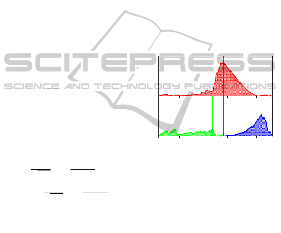
To find the best segment boundary t
∗
to cut x into
two segments, we run through all t, and pick t = t
∗
such that
∆
max
= ∆(t
∗
) = max
t
∆(t), (4)
as shown in Figure 2. At t = t
∗
, the left and right seg-
ments are the most distinct statistically. We call ∆(t
∗
)
the strength of the segment boundary at t = t
∗
. To find
more segment boundaries, we repeat this one-to-two
segmentation procedure for x
L
and x
R
, and all sub-
sequent segments. As the segments get shorter, the
divergence maxima of new segment boundaries will
also get smaller. When these divergence maxima be-
come too small, the new segment boundaries will no
longer be statistically significant. Further segmenta-
tion thus becomes meaningless.
1997 1998 1999 2000 2001 2002 2003 2004
2005 2006
2007 2008
0
500
1000
1500
2000
Jensen-Shannon divergence
0
500
1000
1500
2000
2500
(a)
(b)
Figure 2: Jensen-Shannon divergence spectrum of the Dow
Jones Industrial Average index time series between January
1997 and August 2008 (red), based on which we identify (a)
the first segment boundary to be around the middle of 2003
(marked by red vertical line). To further segment the left
and right subsequences, we compute the Jensen-Shannon
divergence spectra (green and blue respectively) entirely
within the respective subsequences, and (b) find the loca-
tions of their divergence maxima.
There are three approaches to terminating the re-
cursive segmentation in the literature. In the orig-
inal approach by Bernaola-Galv
´
an and coworkers
(Bernaola-Galv
´
an et al., 1996; Rom
´
an-Rold
´
an et al.,
1998), the divergence maximum of a new segment
boundary is tested for statistical significance against
a χ
2
distribution whose degree of freedom depends
on the length of the segment to be subdivided. Recur-
sive segmentation terminates when no new segment
boundaries more significant than the chosen confi-
dence level can be found. In the second approach
(Li, 2001b; Li, 2001a), a segment is subdivided
if the information criterion of its best two-segment
model exceeds that of its one-segment model. Re-
cursive segmentation terminates when further seg-
KDIR 2011 - International Conference on Knowledge Discovery and Information Retrieval
54

mentation does not explain the data better. In the
third approach (Cheong et al., 2009b), we compare
the Jensen-Shannon divergence ∆(t) against a coarse-
grained divergence
˜
∆(t) of the segment to be subdi-
vided, to compute the total strength of point-to-point
fluctuations in ∆(t). Recursive segmentation termi-
nates when the area under
˜
∆(t) falls below the desired
signal-to-noise ratio. The most statistically significant
segment boundaries will all be discovered using any
of the three termination criteria.
Based on the experience in our previous work
(Wong et al., 2009), these most statistically signifi-
cant segment boundaries are also discovered if we ter-
minate the recursive segmentation when no new opti-
mized segment boundaries with Jensen-Shannon di-
vergence greater than a cutoff of ∆
0
= 10 are found.
This simple termination criterion sometimes result in
long segments whose internal segment structures are
masked by their contexts (Cheong et al., 2009a). For
these long segments, we progressively lower the cut-
off ∆
0
until a segment boundary with strength ∆ > 10
appears. The final segmentation then consists of seg-
ment boundaries discovered through the automated
recursive segmentation, as well as segment bound-
aries discovered through progressive refinement of
overly long segments.
At each stage of the recursive segmentation, we
also perform segmentation optimization, using the al-
gorithm described in Cheong et al. (2009b). Given M
segment boundaries {t
1
,. . . ,t
M
}, some of which are
old, and some of which are new, we optimize the po-
sition of the mth segment boundary by computing the
Jensen-Shannon divergence spectrum within the su-
persegment bounded by the segment boundaries t
m−1
and t
m+1
, and replace t
m
by t
∗
m
, where the superseg-
ment Jensen-Shannon divergence is maximized. We
do this iteratively for all M segment boundaries, until
all segment boundaries converge to their optimal po-
sitions. This optimization step is necessary, because
of the context sensitivity problem discussed in Cheong
et al. (2009a). Otherwise, statistically significant seg-
ment boundaries are likely to be masked by the con-
text they are embedded within, and missed by the seg-
mentation procedure.
2.2 Hierarchical Clustering
After the recursive segmentation terminates, we typi-
cally end up with a large number of segments. Neigh-
boring segments are statistically distinct, but might be
statistically similar to distant segments. We can group
statistically similar segments together, to estimate the
number P of time series segment classes. Various sta-
tistical clustering schemes can be used to achieve this
(see for example, the review by Jain, Murty and Flynn
(Jain et al., 1999), or texts on unsupervised machine
learning). Since the number of clusters is not known
beforehand, we chose to perform agglomerative hier-
archical clustering, using the complete link algorithm.
The statistical distances between segments are given
by their Jensen-Shannon divergences.
93
95
98
103
90
31.3
1
104
14
16
46
8
87
92
5
20
82
3
100
97
17
94
89
22
84
78
739.1
4
112
30
10
40
44
15
80
19
49
86
64
66
68
27
32
88
102
81
105
83
75
91
96
249.3
42.7
6
85
99
55
39
65
52
54
77
29
107
115
2
67
61
74
11
57
47
23
50
33
41
31
38
45
7
26
21
73
79
43
56
63
13
34
18
59
62
69
114
116
71
109
111
102.2
34.4
9
53
25
110
48
60
12
35
58
24
101
36
42
106
51
72
28
76
37
108
70
113
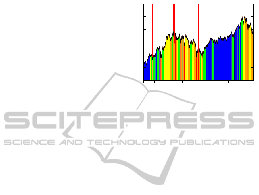
Figure 3: The complete-link hierarchical clustering tree of
the Dow Jones Industrial Average index time series seg-
ments assuming that the index movements within each seg-
ment are normally distributed. The differentiated clusters
are coloured according to their standard deviations: low
(deep blue and blue), moderate (green), high (yellow and
orange), and extremely high (red). Also shown at the ma-
jor branches are the Jensen-Shannon divergence values at
which subclusters are merged.
In Figure 3, we show the hierarchical clustering
tree for the Dow Jones Industrial Average index time
series segments, which tells us the following. If we
select a global threshold ∆ > 739.1, we end up with
one cluster, whereas if we select a global threshold
249.3 < ∆ < 739.1, we find two clusters. These clus-
ters are statistically robust, because they are not sen-
sitive to small variations of the global threshold ∆.
However, they are not as informative as we would
like them to be. Going to a lower global threshold
of ∆ = 30, we find seven clusters. These seven clus-
ters give us a more informative dynamical picture, but
some of the clusters are not robust. If instead of a
global threshold for all robust clusters, we allow local
thresholds, i.e. ∆ = 30 to differentiate the deep blue
and blue clusters, the green and yellow clusters, and
∆ = 40 to differentiate the orange and red clusters, we
will find six natural and robust clusters.
These clusters are differentiated by their standard
deviations, with deep blue being the lowest, and red
being the highest. Based on the actual magnitudes
of the standard deviations (also called market volatili-
ties in the finance literature), we can also group the
time series segments into four clusters: low (deep
TIME SERIES SEGMENTATION AS A DISCOVERY TOOL - A Case Study of the US and Japanese Financial Markets
55

blue and blue), moderate (green), high (yellow and
orange), and extremely high (red). As we will ex-
plain in Section 3, these four clusters have very natu-
ral interpretations as the growth (low-volatility), cor-
rection (moderate-volatility), crisis (high-volatility),
and crash (extremely-high-volatility) macroeconomic
phases.
2.3 Validation against Synthetic Data
To test the segmentation scheme, we perform several
numerical experiments on artificial Gaussian time se-
ries. First, we set the standard deviations of the two
5,000-long segments to σ
L
= σ
R
= 1.0. We also fix
the mean of the left segment at µ
L
= 0, and vary the
mean µ
R
of the right segment. As we can see from
Table 1(a), the segmentation scheme found only the
single segment boundary at t
∗
= 5000, for a differ-
ence in mean as small as ∆µ = |µ
L
−µ
R
| = 0.1. This
is remarkable, because the standard deviations of both
segments are σ
L
= σ
R
= 1.0 > ∆µ. As expected,
the standard error for the boundary position decreases
with increasing ∆µ.
Table 1: Positions and standard errors of the segment
boundary discovered using the Jensen-Shannon divergence
segmentation scheme, from 1,000 artificial Gaussian time
series. In (a) and (b), we set N
L
= N
R
= 5, 000, (µ
L
,σ
L
) =
(0,1), σ
R
= 1, and vary µ
R
. In (b), we set N
L
= N
R
= 5,000,
(µ
L
,σ
L
) = (0, 1), µ
R
= 0, and vary σ
R
. In (c), we set
(µ
L
,σ
L
) = (0,1), (µ
R
= 0, σ
R
) = (0,0.5), and vary N =
N
L
+ N
R
.
(a)
µ
R
t
∗
±∆t
∗
0.1 4990 ±680
0.2 4980 ±500
0.5 5000 ±490
1.0 4990 ±260
2.0 5010 ±330
5.0 5020 ±410
10.0 5000 ±270
(b)
σ
2
t
∗
±∆t
∗
0.1 5000 ±380
0.2 5000 ±350
0.3 5010 ±480
0.4 5020 ±420
0.5 5000 ±280
0.7 5010 ±320
0.9 5000 ±550
(c)
N t
∗
±∆t
∗
100 49 ±7
200 98 ±9
500 249 ±15
1000 497 ±41
2000 998 ±28
5000 2500 ±200
10000 5000 ±290
Next, we set µ
L
= µ
R
= 0, fix σ
L
= 1.0, and vary
σ
R
. Again, as we can see from Table 1(b), the single
boundary at t
∗
= 5000 was found for ratio of stan-
dard deviations as close to one as σ
R
/σ
L
= 0.9. As
expected, the standard error for the boundary position
decreases with increasing disparity between σ
L
and
σ
R
. Finally, we set (µ
L
,σ
L
) = (0,1) and (µ
R
,σ
R
) =
(0,0.5), and vary the length N of the artificial time
series, always keeping the segment boundary in the
middle. From Table 1(c), we see that the boundary
position is very accurately determined for time series
as short as N = 100. We also see the standard error
growing much slower than N.
Following this, we recursively segmented 10,000
artificial Gaussian time series of length N = 1000,
each consisting of the same 10 segments shown in Ta-
ble 2. We also see in Table 2 that eight of the nine seg-
ment boundaries were accurately determined. The po-
sition of the remaining boundary, between segments
m = 4 and m = 5, has a large standard error because
it separates two segments that are very similar statis-
tically.
Table 2: The ten segments of the N = 10,000 artificial
Gaussian time series, and the segment boundaries obtained
using the recursive Jensen-Shannon divergence segmenta-
tion scheme.
m start end µ
m
σ
m
t
∗
±∆t
∗
1 1 1500 0.55 0.275 1497 ±60
2 1501 2500 0.05 0.025 2500 ±14
3 2501 3500 0.20 0.10 3504 ±50
4 3501 5000 0.60 0.30 5010 ±140
5 5001 6501 0.65 0.325 6497 ±39
6 6501 7000 0.30 0.15 7002 ±26
7 7001 8500 0.45 0.225 8500 ±12
8 8501 9000 0.05 0.025 9001 ±12
9 9001 9500 0.45 0.225 9500 ±9
10 9501 10000 0.15 0.075 -
Finally, we timed the MATLAB code that we used
to implement the recursive segmentation. The spatial
complexity of this scheme is O(N), since we need to
store the original time series and two other processed
data arrays of the same length. The temporal com-
plexity of the scheme, however, cannot be easily an-
alyzed, because it depends on how many optimiza-
tion iterations are needed, and how many segment
boundaries are to be discovered. On a MacBook Pro
with 2.4-GHz core-2 duo and 4-GB 1067-MHz DDR3
memory, the two-segment time series took 1±1 ms to
segment, for N = 100, and 63 ±5 ms to segment, for
N = 10000. The 10-segment time series with length
N = 10,000 took 0.38 ±0.03 s to segment, or 42 ±3
ms for each boundary. We also segmented 30 50,000-
point time series from a molecular dynamics simula-
tion of penta-analine. 7084 boundaries were found
after 114 s, which works out to 16 ms per boundary.
KDIR 2011 - International Conference on Knowledge Discovery and Information Retrieval
56
3 CASE STUDY
3.1 Single US Time Series
For the single time series study, we chose the Dow
Jones Industrial Average (DJI) index. This is a
price-weighted average of the stock prices of the
30 most well capitalized US companies. Tic-by-tic
data between 1 January 1997 and 31 August 2008
for this index was downloaded from the Thomson-
Reuters Tickhistory database (formerly SIRCA
Taqtic, https://tickhistory.thomsonreuters.
com/TickHistory/login.jsp), and processed into
a half-hourly index time series X = (X
1
,X
2
,. . . ,X
N
).
From X, we then obtain the half-hourly index move-
ment time series x = (x
1
,x
2
,. . . ,x
n
), where x
t
=
X
t+1
−X
t
and n = N −1, which we assume consists of
M statistically stationary segments. The half-hourly
data frequency was chosen so that we can reliably
identify segments as short as a single day. We do not
go to higher data frequencies, because we are not in-
terested in intraday segments.
As reported in Wong et al. (2009), the clustered
segments of the DJI tell very interesting stories when
we plot how they are distributed over the January
1997 to August 2008 period. From Figure 4, we see
that the DJI (as a proxy for the US economy as a
whole) spends most of its time in the low-volatility
phase (dark blue and blue) and the high-volatility
phase (yellow and orange). Based on when it oc-
curs, we can associate the low-volatility phase with
economic expansion. We also see that the previous
March to November 2001 economic contraction for
the US is completely nested within the high-volatility
phase. This suggests that the high-volatility phase
has the natural interpretation as an economic crisis
phase, which lasts longer than most official reces-
sions. Interrupting both the low-volatility and high-
volatility phases, we also find short-lived moderate-
volatility phases (green), which we can therefore
interpret as market corrections. In addition, even
shorter-lived extreme-high-volatility phases (red) can
be found almost exclusively within the high-volatility
phase. These can be unambiguously associated with
market crashes.
More importantly, the temporal distribution tells
us that the US economy, as measured by the DJI, went
into a five-year crisis period starting in mid-1998, be-
fore recovering in mid-2003. The US economy then
enjoyed a remarkable four-year period of sustained
growth, before succumbing to the Subprime Crisis in
mid-2007. We also see in the temporal distribution the
existence of year-long series of precursor shocks pre-
ceding each transition. These precursor shocks sug-
1997 1998 1999 2000 2001 2002 2003 2004
2005 2006
2007 2008
4000
6000
8000
10000
12000
14000
16000
DJI
1 2 3 4 5 6 7 8 9 10
Figure 4: Temporal distributions of the clustered segments
superimposed onto the DJI time series. The red solid lines
indicate the dates of important market events: (1) July 1997
Asian Financial Crisis; (2) October 1997 Mini Crash; (3)
August 1998 Russian Financial Crisis; (4) DJI 2000 High;
(5) NASDAQ Crash; (6) start of 2001 recession; (7) Sep 11
Attack; (8) end of 2001 recession; (9) DJI 2002 Low; (10)
February 2007 Chinese Correction.
gest on the surface that the July 1997 Asian Finan-
cial Crisis triggered the previous crisis, whereas mar-
ket corrections in the Chinese markets, which started
in May 2006, triggered the present crisis. Further-
more, the mid-2003 economic recovery is preceded
by a year-long series of inverted shocks after the 2002
lows. Therefore, if the fundamental dynamics behind
the US economy had not changed from 2002 to 2009,
we expect from this single time series study that the
US economy will emerge from the global financial
crisis one year after the March 2009 lows, i.e. shortly
after the first quarter of 2010. In contrast, the US
National Bureau of Economic Research (NBER) an-
nounced in Sep 2010 that the US economic recession
ended in Jun 2009.
3.2 Cross Section of US Time Series
The story of the US economy becomes even richer
and more interesting, when we do a comparative seg-
mentation and clustering analysis of the ten Dow
Jones US (DJUS) economic sector indices (Lee et al.,
2009). Tic-by-tic data between 14 Feb 2000 and
31 Aug 2008 for these ten indices (see Table 3)
were downloaded from the Thomson-Reuters Tick-
History database. Since different indices have differ-
ent magnitudes, we processed the raw data first into
half-hourly time series X
i
= (X
i,1
,X
i,2
,. . . ,X
i,N
) for
each of the ten indices i = 1, . ..,10, before obtain-
ing the half-hourly log-index movement time series
y
i
= (y
i,1
,y
i,2
,. . . ,y
i,n
), i = 1,...,10, n = N −1, where
y
i,t
= ln X
i,t+1
−lnX
i,t
for more meaningful compari-
TIME SERIES SEGMENTATION AS A DISCOVERY TOOL - A Case Study of the US and Japanese Financial Markets
57
son between the indices.
Table 3: The ten Dow Jones US economic sector indices.
i symbol sector
1 BM Basic Materials
2 CY Consumer Services
3 EN Energy
4 FN Financials
5 HC Healthcare
6 IN Industrials
7 NC Consumer Goods
8 TC Technology
9 TL Telecommunications
10 UT Utilities
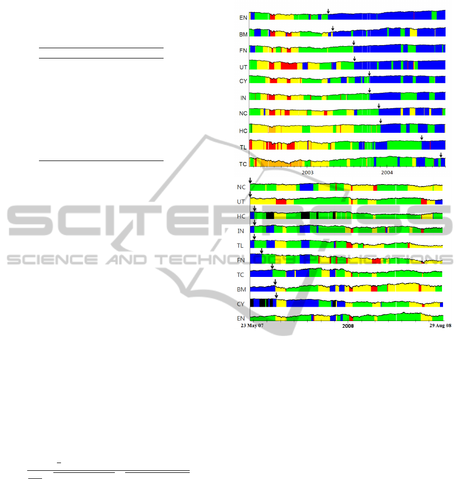
The first interesting observation we make is that
the time it takes for the US economy to recover from
a financial crisis (one-and-a-half years, Figure 5(a))
and that for it to completely enter a financial crisis
(two months, Figure 5(b)) are very different in scale.
For the mid-2003 US economic recovery, the first two
sectors to recover are EN and BM, and the last two
sectors to recover are TL and TC. It is reasonable for
EN and BM to recover first, since they are at the base
of the economic supply chain. It is also reasonable
that TC and TL were the last sectors to recover, since
the previous financial crisis was the result of the tech-
nology bubble bursting. For the mid-2007 US eco-
nomic decline, we find some surprises: instead of NC
(which includes homebuilders and realties) and FN
(which includes banks) being responsible for drag-
ging the US economy down, fully half of the DJUS
economic sectors entered the crisis phase before FN.
Guided by this coarse-grained picture of the US
economy’s slow time evolution, we can extract even
more understanding from the high-frequency fluctua-
tions (Zhang et al., 2011). We do this by computing
the linear cross correlations
C
i j
=
1
n
∑
n
t=1
(y
i,t
− ¯y
i
)(y
j,t
− ¯y
j
)
1
n−1
p
∑
n
t=1
(y
i,t
− ¯y
i
)
2
p
∑
n
t=1
(y
j,t
− ¯y
j
)
2
(5)
between the ten DJUS economic sector indices over
different time intervals. We then look at the mini-
mal spanning tree (MST) representation of the cross-
correlation matrix (Kruskal, 1956; Prim, 1957; Man-
tegna, 1999). The MST shows only the nine strongest
links that do not incorporate cycles into the graph of
the ten US economic sectors.
In this part of our study, we computed the cross-
correlation matrix first over the entire time series,
from February 2000 to August 2008. From Figure
6(a), we see that IN, CY and NC, are at the centre of
the MST, while the sectors HC, TC, TL, and UT lie
on the fringe of the MST. This is consistent with the
Figure 5: Temporal distributions of clustered segments for
the time series of all ten US economic sectors (top) between
April 2002 and September 2004, showing the sequence of
recovery from the mid-1998 to mid-2003 financial crisis,
and (bottom) between 23 May 2007 and 29 August 2008,
showing the sequence of descent into the present financial
crisis.
former group of sectors being of central importance,
and the latter being of lesser importance to the US
economy (Heimo et al., 2009).
We also expect interesting structural differences
between MSTs constructed entirely within the pre-
vious crisis (2001–2002, Figure 6(b)), the previous
growth (2004–2005, Figure 6(c)), and the present cri-
sis (2008–2009, Figure 6(d)). Indeed, we see two dis-
tinct MST topologies: a chain-like MST which occurs
for both crises, and a star-like MST which occurs for
the growth phase. Even though we only have three
data points (two crises and a growth), we believe the
generic association of chain-like MST and star-like
MST to the crisis and growth phases respectively is
statistically robust. Our assessment that the topology
change in the MST is statistically significant is further
supported by the observations by Onnela et al., at the
microscopic scale of individual stocks (Onnela et al.,
2003a; Onnela et al., 2003b; Onnela et al., 2003c).
KDIR 2011 - International Conference on Knowledge Discovery and Information Retrieval
58
EN BM IN
TC
TL
CY
FN
NC
UT
HC
(a)
BM IN
TC
ENUT
FN
CY
NC HC
TL
(b)
IN
TC
EN BM
FN TL
UT
HC
CY
NC
(c)
BM IN
TC
EN HCNCCY
TL
FN UT
(d)
Figure 6: The MSTs of the ten DJUS economic sectors,
constructed using half-hourly time series from (a) February
2000 to August 2008, (b) 2001–2002, (c) 2004–2005, and
(d) 2008-2009. The first and the third two-year windows,
(b) and (d), are entirely within an economic crisis, whereas
the second two-year window, (c), is entirely within an eco-
nomic growth period.
IN
TC
EN BM
FN TL
UT
HC
CY
NC
INEN BM NC
FN
HC
TL
TC
CY UT
(a) (b)
Figure 7: Comparison of the MSTs for (a) the 2004–
2005 growth period, and (b) the moderate-volatility seg-
ment around September 2009.
Speaking of ‘green shoots’ of economic revival
that were evident in Mar 2009, Federal Reserve chair-
man Ben Bernanke predicted that “America’s worst
recession in decades will likely end in 2009 before a
recovery gathers steam in 2010”. We therefore looked
out for a star-like MST in the time series data of 2009
and 2010. Star-like MSTs can also be found deep in-
side an economic crisis phase, but they very quickly
unravel to become chain-like MSTs. A persistent star-
like MST, if it can be found, is statistical signature
that the US economy is firmly on track to full re-
covery (which may take up to two years across all
sectors). More importantly, the closer the MST of a
given period is to a star, the closer we are to the ac-
tual recovery. Indeed, the MST is already star-like for
a moderate-volatility segment in Sep 2009 (see Fig-
ure 7), and stayed robustly star-like throughout the
Greek Debt Crisis of May/Jun 2010. The statistical
evidence thus suggests that the US economy started
recovering late 2009, and stayed the course through
2010. Bernanke was indeed prophetic.
3.3 Cross Section of Japanese Time
Series
As a comparison, we also segmented the 36 Nikkei
500 Japanese industry indices (see Table 4) between
1 Jan 1996 and 11 Jun 2010. Tic-by-tic data were
downloaded from the Thomson-Reuters TickHistory
database, and processed into half-hourly index time
series X
i
= {X
i,1
,X
i,2
,. . . ,X
i,N
}, i = 1, . . .,36. As
with the US cross section study, we then obtain
the half-hourly log-index movement time series y
i
=
(y
i,1
,y
i,2
,. . . ,y
i,n
), i = 1,...,36, n = N − 1, where
y
i,t
= ln X
i,t+1
−ln X
i,t
for more meaningful compar-
ison between the indices.
2002
2003
2004
2005 2006
2007
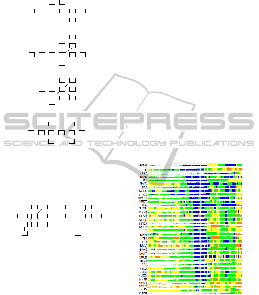
Figure 8: Temporal distributions of the 36 Nikkei 500
Japanese industry indices from January 2002 to December
2007. In this figure, the growth segments are colored blue,
correction segments are colored green, crisis segments are
colored yellow or orange, and crash segments are colored
red.
In this paper, we will focus on the 2005 near re-
covery of the Japanese economy, and the 2007 fall of
TIME SERIES SEGMENTATION AS A DISCOVERY TOOL - A Case Study of the US and Japanese Financial Markets
59
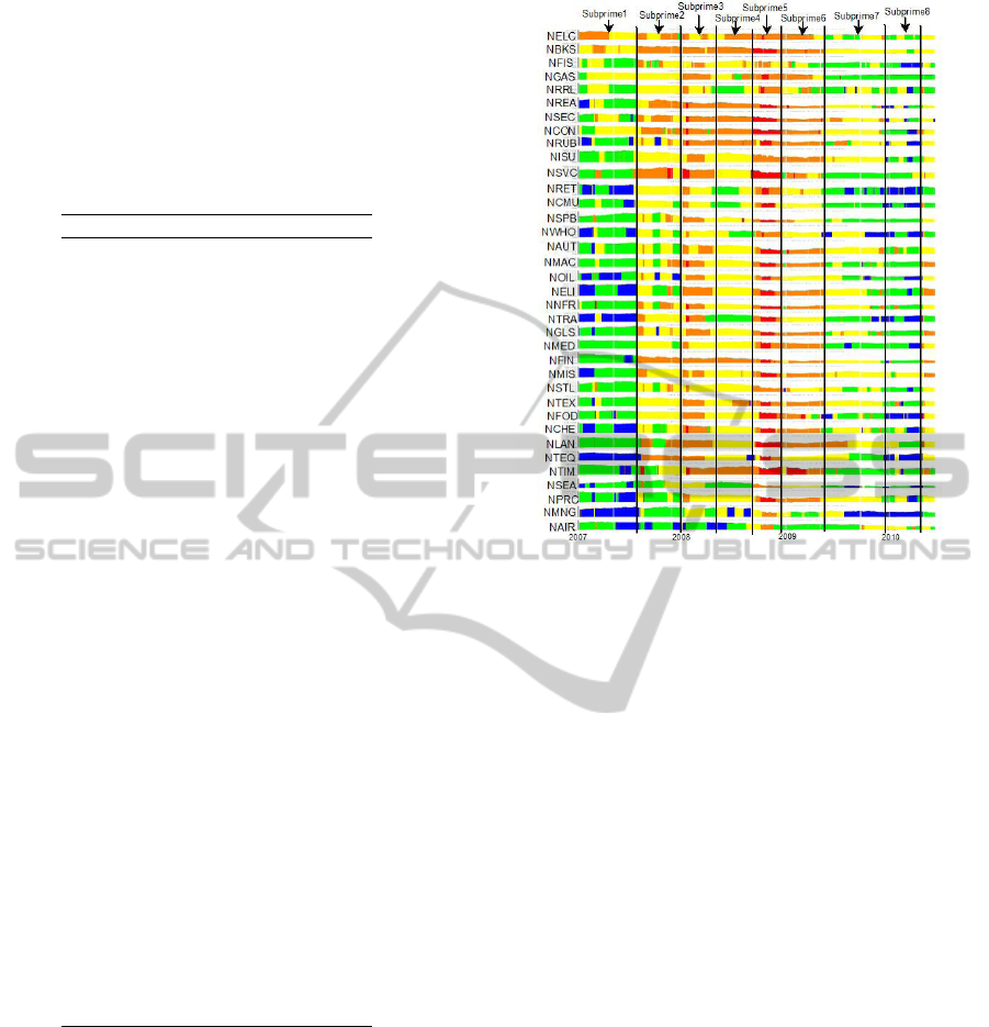
Table 4: The 36 Nikkei 500 industry indices. Each index is
a price-weighted average of stocks which are components of
the Nikkei 500 index. The Nikkei 500 index was first cal-
culated on January 4, 1972 with a value of 223.70, and its
500 component stocks are selected from the first section of
the Tokyo Stock Exchange based on trading volume, trad-
ing value and market capitalization for the preceding three
years. The makeup of the Nikkei 500 is reviewed yearly,
and each year approximately 30 stocks are replaced.
i symbol industry
1 NAIR Air Transport
2 NAUT Automotive
3 NBKS Banking
4 NCHE Chemicals
5 NCMU Communications
6 NCON Construction
7 NELC Electric Power
8 NELI Electric Machinery
9 NFIN Other Financial Services
10 NFIS Fisheries
11 NFOD Foods
12 NGAS Gas
13 NGLS Glass & Ceramics
14 NISU Insurance
15 NLAN Other Land Transport
16 NMAC Machinery
17 NMED Pharmaceuticals
18 NMIS Other Manufacturing
19 NMNG Mining
20 NNFR Nonferrous Metals
21 NOIL Oil & Coal Products
22 NPRC Precision Instruments
23 NREA Real Estate
24 NRET Retail
25 NRRL Railway/Bus
26 NRUB Rubber Products
27 NSEA Marine Transport
28 NSEC Securities
29 NSPB Shipbuilding
30 NSTL Steel Products
31 NSVC Services
32 NTEQ Other Transport Equipment
33 NTEX Textiles & Apparel
34 NTIM Pulp & Paper
35 NTRA Trading Companies
36 NWHO Warehousing
the Japanese economy to the Subprime Crisis. From
Figure 8, we see that NMNG started growing the ear-
liest, NFIS started growing the latest, while NSPB did
not seem to have grown at all between 2002 and 2005.
We see also that the Japanese economy, led by NMNG
and NELC, took two years and two months to com-
pletely recover from the back-to-back Asian Financial
and Technology Bubble Crises. While the time scales
of complete economic recovery appear to be differ-
ent, very similar industries led the recovery processes
of US and Japan.
Next, we look at how the Japanese economy suc-
Figure 9: Temporal distributions of the 36 Nikkei 500
Japanese industry indices from January 2007 to June 2010.
In this figure, the growth segments are colored blue, cor-
rection segments are colored green, crisis segments are col-
ored yellow or orange, and crash segments are colored red.
Within this period, we can identify eight corresponding seg-
ments, labeled ‘Subprime1’ to ‘Subprime8’.
cumbed to the Subprime Crisis. As we can see from
Figure 9, the Japanese economy fell in five stages.
The most important time scale in Japan’s response
to the Subprime Crisis is that associated with stage
2, which appears to be triggered by the start of the
Subprime Crisis in US, and affected 21 out of 36
Nikkei 500 industries. Here, the Subprime Crisis
swept through NISU, NSVC, NRUB to NTEQ in a
mere 27 days. This is half the time it took for the US
economy to fall from first to the last economic sector,
with NC (the sector homebuilders belong to) leading
the pack. As late as June 2010, most Japanese in-
dustries were still in the sustained crisis phase. Only
NMNG, NWHO, NTRA, and NRET showed signs
of early recovery from mid 2009 onwards. If the
Japanese economy again takes two and a half years
to completely recover, this will happen in the begin-
ning of 2012.
Finally, we tracked how the MST change going
from one segment to the next during the Subprime
Crisis. In 21st century Japanese economy, NELI,
NMAC, and NCHE are the growth industries, based
on the fact that they are hubs consistently in all or
most of the MSTs. NNFR and NRRL, which we con-
sider quality industries, also become occasional hubs
KDIR 2011 - International Conference on Knowledge Discovery and Information Retrieval
60

in the MSTs. In Figure 10, we see the NNFR and
NRRL clusters of industries growing at the expense
of the NCHE and NMAC clusters of industries, as we
go from the Subprime3 period to the Subprime4 pe-
riod. This tells us that the pheripheral industries went
from being most strongly correlated with NCHE and
NMAC to being most strongly correlated with NNFR
and NRRL. We believe this is a signature of money
leaving the NCHE and NMAC industries, and enter-
ing the NNFR and NRRL industries, i.e. a flight to
quality (Connolly et al., 2005; Baur and Lucey, 2009)
from NCHE/NMAC to NNFR/NRRL.
(a)
(b)
Figure 10: MSTs for the (a) Subprime3 period and (b) Sub-
prime4 period. In this figure, the number beside each link
indicates the order in which the link was added to the MST,
whereas the thicknesses of the links indicate how strong the
correlations are between industries.
4 CONCLUSIONS
To conclude, we have explained how the dynamics
of complex systems self-organize to reside on low-
dimensional manifolds governed by the slow time
evolution of a small set of effective variables. We ex-
plained how these low-dimensional manifolds are re-
lated to thermodynamic phases, how fast fluctuations
of microscopic variables are dictated by which low-
dimensional manifold the system is in. We then ex-
plained how it is possible to discover the phases of a
complex system by statistically classifying the micro-
scopic time series, each class representing a macro-
scopic phase.
Following this, we described in details the time
series segmentation method adapted from the origi-
nal scheme developed by Bernaola-Galv
´
an et al. for
biological sequence segmentation. In this method,
we examine the Jensen-Shannon divergence spectrum
∆(t) of the given time series, to see how much bet-
ter the data is fitted by two distinct stochastic mod-
els than it is by one stochastic model. The time se-
ries will then be cut into two segments at the point
where ∆(t) is maximized. This one-to-two segmen-
tation is then applied recursively to obtain more and
more segments. At each stage of the recursive seg-
mentation, we optimize the positions of all segment
boundaries. The recursive segmentation is terminated
when the strengths of new segment boundaries fall
below the chose threshold of ∆
0
= 10. Long seg-
ments are then progressively refined, before we per-
form complete-link hierarchical clustering on the time
series segments to discover the natural number of time
series segment classes.
After a systematic test of the method on artificial
time series, we performed time series segmentation
on the Dow Jones Industrial Average index time se-
ries, the ten Dow Jones US Economic Sector indices,
and the 36 Nikkei 500 Japanese Industry indices, as
a concrete demonstration of its potential for knowl-
edge discovery. From the single time series study,
we found the time series segments very naturally fall
into four to six clusters, which can be roughly asso-
ciated with the growth, crisis, correction, and crash
macroeconomic phases. We also measured the life-
times of the previous US crisis and growth phases to
be about five years and four years respectively. From
cross section studies, we found that the US economy
took one-and-a-half years to completely recover from
the Technology Bubble Crisis, but only two months to
completely succumb to the Subprime Crisis. In con-
trast, the Japanese economy took two years and two
months to completely recover from the previous cri-
sis, and only 27 days for the Subprime Crisis to com-
pletely set in. For both countries, the previous eco-
nomic recoveries were led by industries at the base of
the economic supply chain.
Guided by the time series segments, we also
analyzed the cross correlations within the US and
Japanese financial markets, visualizing these in terms
of MSTs. The MST visualizations allowed us to iden-
tify IN, CY, and NC, NCHE, NELI, and NMAC, to
be the cores of the US and Japanese economies re-
spectively. We detected an early recovery for the US
economy in late 2009, based on the star-like MST
seen at this time. We concluded that the US recovery
TIME SERIES SEGMENTATION AS A DISCOVERY TOOL - A Case Study of the US and Japanese Financial Markets
61

gained strength, as the MST remained robustly star-
like through the first half of 2010. For the Japanese
economy, we identified flights to quality within the
financial markets, and also the lack of clear signs of
recovery as late as Jun 2010.
ACKNOWLEDGEMENTS
This research is supported by startup grant SUG 19/07
from the Nanyang Technological University. RPF
and DYX thank the Nanyang Technological Univer-
sity Summer Research Internship Programme for fi-
nancial support during Jun and Jul 2010.
REFERENCES
Barranco-L
´
opez, V., Luque-Escamilla, P., Mart
´
ınez-Aroza,
J., and Rom
´
an-Rold
´
an, R. (1995). Entropic texture-
edge detection for image segmentation. Electronic
Letters, 31:867–869.
Baur, D. G. and Lucey, B. M. (2009). Flights and contagion
— an empirical analysis of stock-bond correlations.
Journal of Financial Stability, 5(4):339–352.
Bernaola-Galv
´
an, P., Ivanov, P. C., Amaral, L. A. N., and
Stanley, H. E. (2001). Scale invariance in the nonsta-
tionarity of human heart rate. Physical Review Letters,
87:168105.
Bernaola-Galv
´
an, P., Rom
´
an-Rold
´
an, R., and Oliver, J. L.
(1996). Compositional segmentation and long-range
fractal correlations in dna sequences. Physical Review
E, 53(5):5181–5189.
Bialonski, S. and Lehnertz, K. (2006). Identifying phase
synchronization clusters in spatially extended dynam-
ical systems. Physical Review E, 74:051909.
Bivona, S., Bonanno, G., Burlon, R., Gurrera, D., and
Leone, C. (2008). Taxonomy of correlations of wind
velocity — an application to the sicilian area. Physica
A, 387:5910–5915.
Braun, J. V., Braun, R. K., and M
¨
uller, H.-G. (2000). Mul-
tiple changepoint fitting via quasilikelihood, with ap-
plication to dna sequence segmentation. Biometrika,
87(2):301–314.
Braun, J. V. and M
¨
uller, H.-G. (1998). Statistical methods
for dna sequence segmentation. Statistical Science,
13(2):142–162.
Carlstein, E. G., M
¨
uller, H.-G., and Siegmund, D. (1994).
Change-Point Problems, volume 23 of Lecture Notes-
Monograph Series. Institute of Mathematical Statis-
tics.
Chen, J. and Gupta, A. K. (2000). Parametric Statistical
Change Point Analysis. Birkh
¨
auser.
Cheong, S.-A., Stodghill, P., Schneider, D. J., Cartinhour,
S. W., and Myers, C. R. (2009a). The context sen-
sitivity problem in biological sequence segmentation.
q-bio/0904.2668.
Cheong, S.-A., Stodghill, P., Schneider, D. J., Cartinhour,
S. W., and Myers, C. R. (2009b). Extending the re-
cursive jensen-shannon segmentation of biological se-
quences. q-bio/0904.2466.
Chung, F.-L., Fu, T.-C., Luk, R., and Ng, V. (2002). Evo-
lutionary time series segmentation for stock data min-
ing. In Proceedings of the IEEE International Confer-
ence on Data Mining 2002 (9–12 Dec 2002, Maebashi
City, Japan), pages 83–90.
Churchill, G. A. (1989). Stochastic models for heteroge-
neous dna sequences. Bulletin of Mathematical Biol-
ogy, 51(1):79–94.
Churchill, G. A. (1992). Hidden markov chains and the
analysis of genome structure. Computers & Chem-
istry, 16(2):107–115.
Connolly, R., Stivers, C., and Sun, L. (2005). Stock
market uncertainty and the stock-bond return rela-
tion. Journal of Financial and Quantitative Analysis,
40(1):161–194.
Crotty, J. (2009). Structural causes of the global finan-
cial crisis: a critical assessment of the ‘new finan-
cial architecture’. Cambridge Journal of Economics,
33(4):563–580.
Dincer, I. (2000). Renewable energy and sustainable devel-
opment: a crucial review. Renewable and Sustainable
Energy Reviews, 4(2):157–175.
Fellman, P. V. (2008). The complexity of terrorist networks.
In Proceedings of the 12th International Conference
on Information Visualization (Jul 9–11, 2008).
Garnaut, R. (2008). The Garnaut Climate Change Review.
Cambridge University Press.
Giorgi, F. and Mearns, L. O. (1991). Approaches to the sim-
ulation of regional climate change: A review. Reviews
of Geophysics, 29(2):191–216.
Goldfeld, S. M. and Quandt, R. E. (1973). A markov model
for switching regressions. Journal of Econometrics,
1:3–16.
Gross, R., Leach, M., and Bauen, A. (2003). Progress
in renewable energy. Environment International,
29(1):105–122.
Hamilton, J. D. (1989). A new approach to the economic
analysis of nonstationary time series and the business
cycle. Econometrica, 57:357–384.
Heimo, T., Kaski, K., and Saram
¨
aki, J. (2009). Maximal
spanning trees, asset graphs and random matrix de-
noising in the analysis of dynamics of financial net-
works. Physica A, 388:145–156.
Jain, A., Murty, M., and Flynn, P. (1999). Data clustering:
A review. ACM Computing Surveys, 31(3):264–323.
Jiang, J., Zhang, Z., and Wang, H. (2007). A new seg-
mentation algorithm to stock time series based on
pip approach. In Proceedings of the Third IEEE In-
ternational Conference on Wireless Communications,
Networking and Mobile Computing 2007 (21–25 Sep
2007, Shanghai, China), pages 5609–5612.
Kruskal, J. B. (1956). On the shortest spanning subtree of
a graph and the traveling salesman problem. Proceed-
ings of the American Mathematical Society, 7:48–50.
KDIR 2011 - International Conference on Knowledge Discovery and Information Retrieval
62

Lai, S. K., Lin, Y. T., Hsu, P. J., and Cheong, S. A. (2011).
Dynamical study of metallic clusters using the sta-
tistical method of time series clustering. Computer
Physics Communications, 182:1013–1026.
Leach, M., Scoones, I., and Stirling, A. (2010). Governing
epidemics in an age of complexity: Narratives, poli-
tics and pathways to sustainability. Global Environ-
mental Change, 20(3):369–377.
Lee, G. H. T., Zhang, Y., Wong, J. C., Prusty, M., and
Cheong, S. A. (2009). Causal links in us economic
sectors. arXiv:0911.4763.
Lee, U. and Kim, S. (2006). Classification of epilepsy types
through global network analysis of scalp electroen-
cephalograms. Physical Review E, 73:041920.
Lemire, D. (2006). Overfitting and time series segmenta-
tion: A locally adaptive solution. arXiv:cs/0605103.
Li, W. (2001a). Dna segmentation as a model selection
process. In Proceedings of the International Confer-
ence on Research in Computational Molecular Biol-
ogy (RECOMB), pages 204–210.
Li, W. (2001b). New stopping criteria for segmenting dna
sequences. Physical Review Letters, 86(25):5815–
5818.
Lin, J. (1991). Divergence measures based on the shannon
entropy. IEEE Transactions on Information Theory,
37(1):145–151.
Mantegna, R. N. (1999). Hierarchical structure in financial
markets. The European Physical Journal B, 11:193–
197.
Monar, J. (2007). The eu’s approach post-september 11:
global terrorism as a multidimensional law enforce-
ment challenge. Cambridge Review of International
Affairs, 20(2):267–283.
Morens, D. M., Folkers, G. K., and Fauci, A. S. (2004).
The challenge of emerging and re-emerging infectious
diseases. Nature, 430:242–249.
Oliver, J. J., Baxter, R. A., and Wallace, C. S. (1998). Min-
imum message length segmentation, volume 1394 of
Lecture Notes in Computer Science, pages 222–233.
Springer.
Onnela, J.-P., Chakraborti, A., Kaski, K., and Kert
´
esz, J.
(2003a). Dynamic asset trees and black monday.
Physica A, 324:247–252.
Onnela, J.-P., Chakraborti, A., Kaski, K., Kert
´
esz, J., and
Kanto, A. (2003b). Asset trees and asset graphs in
financial markets. Physica Scripta, T106:48–54.
Onnela, J.-P., Chakraborti, A., Kaski, K., Kert
´
esz, J., and
Kanto, A. (2003c). Dynamics of market correlations:
Taxonomy and portfolio analysis. Physical Review E,
68(5):056110.
Prim, R. C. (1957). Shortest connection networks and some
generalizations. The Bell System Technical Journal,
36:1389–1401.
Ramensky, V. E., Makeev, V. J., Roytberg, M. A., and Tu-
manyan, V. G. (2000). Dna segmentation through the
bayesian approach. Journal of Computational Biol-
ogy, 7(1–2):215–231.
Rom
´
an-Rold
´
an, R., Bernaola-Galv
´
an, P., and Oliver, J. L.
(1998). Sequence compositional complexity of dna
through an entropic segmentation method. Physical
Review Letters, 80(6):1344–1347.
Santhanam, M. S. and Patra, P. K. (2001). Statistics of atmo-
spheric correlations. Physical Review E, 64:016102.
Taylor, J. B. (2009). The financial crisis and the policy re-
sponses: An empirical analysis of what went wrong.
NBER Working Paper No. 14631.
T
´
oth, B., Lillo, F., and Farmer, J. D. (2010). Segmenta-
tion algorithm for non-stationary compound poisson
processes. The European Physical Journal B - Con-
densed Matter and Complex Systems, 78(2):235–243.
Vaglica, G., Lillo, F., Moro, E., and Mantegna, R. N.
(2008). Scaling laws of strategic behavior and size
heterogeneity in agent dynamics. Physical Review E,
77(3):036110.
Wang, Y., Leung, L. R., McGregor, J. L., Lee, D.-K.,
Wang, W.-C., Ding, Y., and Kimura, F. (2004). Re-
gional climate modeling: Progress, challenges, and
prospects. Journal of the Meteorological Society of
Japan, 82(6):1599–1628.
Wong, J. C., Lian, H., and Cheong, S. A. (2009). Detect-
ing macroeconomic phases in the dow jones industrial
average time series. Physica A, 388(21):4635–4645.
Zhang, Y., Lee, G. H. T., Wong, J. C., Kok, J. L., Prusty,
M., and Cheong, S. A. (2011). Will the us economy
recover in 2010? a minimal spanning tree study. Phys-
ica A, 390(11):2020–2050.
TIME SERIES SEGMENTATION AS A DISCOVERY TOOL - A Case Study of the US and Japanese Financial Markets
63
