
LEARNING METHOD UTILIZING SINGULAR REGION
OF MULTILAYER PERCEPTRON
Ryohei Nakano, Seiya Satoh and Takayuki Ohwaki
Department of Computer Science, Chubu University, 1200 Matsumoto-cho, Kasugai 487-8501, Japan
Keywords:
Multilayer perceptron, Singular region, Learning method, Polynomial network, XOR problem.
Abstract:
In a search space of multilayer perceptron having J hidden units, MLP(J), there exists a singular flat region
created by the projection of the optimal solution of MLP(J−1). Since such a singular region causes serious
slowdown for learning methods, a method for avoiding the region has been aspired. However, such avoiding
does not guarantee the quality of the final solution. This paper proposes a new learning method which does
not avoid but makes good use of singular regions to find a solution good enough for MLP(J). The potential of
the method is shown by our experiments using artificial data sets, XOR problem, and a real data set.
1 INTRODUCTION
It is known in MLP learning that an MLP(J) param-
eter subspace having the same input-output map as
an optimal solution of MLP(J−1) forms a singular
region, and such a singular flat region causes stagna-
tion of learning (Fukumizu and Amari, 2000). Natural
gradient (Amari, 1998; Amari et al., 2000) was once
proposed to avoid such stagnation of MLP learning,
but even the method may get stuck in singular regions
and is not guaranteed to find a good enough solution.
Recently an alternative constructive method has been
proposed (Minnett, 2011).
It is also known that many useful statistical mod-
els, such as MLP, Gaussian mixtures, and HMM, are
singular models having singular regions where pa-
rameters are nonidentifiable. While theoretical re-
search has been vigorously done to clarify mathemat-
ical structure and characteristics of singular models
(Watanabe, 2009), experimental and algorithmic re-
search is rather insufficient to fully support the theo-
ries.
In MLP parameter space there are many local
minima forming equivalence class (Sussmann, 1992).
Even if we exclude equivalence class, it is widely be-
lieved that there still remain local minima (Duda et al.,
2001). When we adopt an exponential function as an
activation function in MLP (Nakano and Saito, 2002),
there surely exist local minima due to the expressive
power of polynomials. In XOR problem, however, it
was proved there is no local minima (Hamey, 1998).
Thus, since we have had no clear knowledge of MLP
parameter space, we usually run a learning method
repeatedly changing initial weights to find a good
enough solution.
This paper proposes a new learning method which
does not avoid but makes good use of singular regions
to find a good enough solution. The method starts
with MLP having one hidden unit and then gradu-
ally increases the number of hidden units until the
intended number. When it increases the number of
hidden units from J−1 to J, it utilizes an optimum
of MLP(J−1) to form the singular region in MLP(J)
parameter space. The singular region forms a line,
and the learning method can descend in the MLP(J)
parameter space since points along the line are sad-
dles. Thus, we can always find a solution of MLP(J)
better than the local minimum of MLP(J−1). Our
method is evaluated by the experiments for sigmoidal
or polynomial-type MLPs using artificial data sets,
XOR problem and a real data set.
Section 2 describes how sigular regions of MLP
can be constructed. Section 3 explains the proposed
method, and Section 4 shows how the method worked
in our experiments.
2 SINGULAR REGION OF
MULTILAYER PERCEPTRON
This section explains how an optimum of MLP(J−1)
can be used to form the singular region in MLP(J)
parameter space (Fukumizu and Amari, 2000). This
106
Nakano R., Satoh S. and Ohwaki T..
LEARNING METHOD UTILIZING SINGULAR REGION OF MULTILAYER PERCEPTRON.
DOI: 10.5220/0003652501060111
In Proceedings of the International Conference on Neural Computation Theory and Applications (NCTA-2011), pages 106-111
ISBN: 978-989-8425-84-3
Copyright
c
2011 SCITEPRESS (Science and Technology Publications, Lda.)

is universal in the sense that it does not depend on the
choice of a target function or an activation function.
Consider the following MLP(J), MLP having
J hidden units and one output unit. Here θ
J
=
{w
0
,w
j
,w
j
, j = 1,...,J}, and w
j
= (w
jk
).
f
J
(x;θ
J
) = w
0
+
J
∑
j=1
w
j
z
j
, z
j
≡ g(w
T
j
x) (1)
Let input vector x = (x
k
) be K-dimensional. Given
training data {(x
µ
,y
µ
),µ = 1,...,N}, we want to find
the parameter vector θ
J
which minimizes the follow-
ing error function.
E
J
=
1
2
N
∑
µ=1
( f
µ
J
− y
µ
)
2
, f
µ
J
≡ f
J
(x
µ
;θ
J
) (2)
At the same time we consider the following
MLP(J−1) having J−1 hidden units, where θ
J−1
=
{u
0
,u
j
,u
j
, j = 2, ..., J}.
f
J−1
(x;θ
J−1
) = u
0
+
J
∑
j=2
u
j
v
j
, v
j
≡ g(u
T
j
x) (3)
For this MLP(J−1) let
b
θ
J−1
denote a critical point
which satisfies the following
∂E
J−1
(θ)
∂θ
= 0.
The necessary conditions for the critical point of MLP
(J−1) are shown below. Here j = 2,...,J, f
µ
J−1
≡
f
J−1
(x
µ
;θ
J−1
), and v
µ
j
≡ g(u
T
j
x
µ
).
∂E
J−1
∂u
0
=
∑
µ
( f
µ
J−1
− y
µ
) = 0
∂E
J−1
∂u
j
=
∑
µ
( f
µ
J−1
− y
µ
) v
µ
j
= 0
∂E
J−1
∂u
j
= u
j
∑
µ
( f
µ
J−1
− y
µ
) g
′
(u
T
j
x
µ
) x
µ
=0
Now we consider the following three reducible pro-
jections α, β, γ, and let
b
Θ
α
J
,
b
Θ
β
J
, and
b
Θ
γ
J
denote the
regions obtained by applying these three projections
to an optimum of MLP(J − 1)
b
θ
J−1
= {bu
0
, bu
j
,bu
j
, j =
2,...,J}.
b
θ
J−1
α
−→
b
Θ
α
J
,
b
θ
J−1
β
−→
b
Θ
β
J
,
b
θ
J−1
γ
−→
b
Θ
γ
J
b
Θ
α
J
≡ {θ
J
| w
0
= bu
0
, w
1
= 0,
w
j
= bu
j
,w
j
= bu
j
, j=2,··· , J} (4)
b
Θ
β
J
≡ {θ
J
| w
0
+ w
1
g(w
10
) = bu
0
,
w
1
=[w
10
,0,··· ,0]
T
,
w
j
= bu
j
,w
j
= bu
j
, j=2,··· , J} (5)
b
Θ
γ
J
≡ {θ
J
| w
0
= bu
0
, w
1
+ w
2
= bu
2
,
w
1
=w
2
=bu
2
,
w
j
= bu
j
,w
j
= bu
j
, j=3,··· , J} (6)
(a) region
b
Θ
α
J
is K-dimensional since free w
1
is a K-
dimensional vector.
(b) region
b
Θ
β
J
is two-dimensional since three free
weights must satisfy the following
w
0
+ w
1
g(w
10
) = bu
0
.
(c) region
b
Θ
γ
is a line since we have only to satisfy
w
1
+ w
2
= bu
2
.
Here we review a critical point where the gradi-
ent ∂E/∂θ of an error function E(θ) gets zero. In the
context of minimization, a critical point is classified
into a local minimum and a saddle. A critical point θ
0
is classified as a local minimum when any point θ in
its neighborhood satisfies E(θ
0
) ≤ E(θ), otherwise is
classified as a saddle.
Now we classify a local minimum into a wok-
bottom and a gutter. A wok-bottom θ
0
is a strict
local minimum where any point θ in its neighbor-
hood satisfies E(θ
0
) < E(θ), and a gutter θ
0
is a point
having a continuous subspace connected to it where
any point θ in the subspace satisfies E(θ) = E(θ
0
) or
E(θ) ≈ E(θ
0
).
The necessary conditions for the critical point of
MLP (J) are shown below. Here j = 2,...,J.
∂E
J
∂w
0
=
∑
µ
( f
µ
J
− y
µ
) = 0
∂E
J
∂w
1
=
∑
µ
( f
µ
J
− y
µ
) z
µ
1
= 0
∂E
J
∂w
j
=
∑
µ
( f
µ
J
− y
µ
) z
µ
j
= 0,
∂E
J
∂w
1
= w
1
∑
µ
( f
µ
J
− y
µ
) g
′
(w
T
1
x
µ
) x
µ
= 0
∂E
J
∂w
j
= w
j
∑
µ
( f
µ
J
− y
µ
) g
′
(w
T
j
x
µ
) x
µ
= 0
Then we check if regions
b
Θ
α
J
,
b
Θ
β
J
, and
b
Θ
γ
J
satisfy
these necessary conditions.
Note that in these regions we have f
µ
J
= f
µ
J−1
and
z
µ
j
= v
µ
j
, j = 2, ..., J. Thus, we see that the first, third,
and fifth equations hold, and the second and fourth
equations are needed to check.
(a) In region
b
Θ
α
J
, since weight vector w
1
is free, the
output of the first hidden unit z
µ
1
is free, which means
it is not guaranteed that the second and fourth equa-
tions hold. Thus,
b
Θ
α
J
is not a singular region.
(b) In region
b
Θ
β
J
, since z
µ
1
(= g(w
10
)) is independent
on µ, the second equation can be reduced to the first
one, and holds. However, the fourth equation does
LEARNING METHOD UTILIZING SINGULAR REGION OF MULTILAYER PERCEPTRON
107

not hold in general unless w
1
= 0. Thus, the follow-
ing area in
b
Θ
β
J
forms a singular region where w
10
is
free.
w
0
= bu
0
, w
1
= 0, w
10
= f ree
w
j
= bu
j
, w
j
= bu
j
, j = 2,...,J
(c) In region
b
Θ
γ
J
, since z
µ
1
= v
µ
2
, the second and fourth
equations hold. Namely,
b
Θ
γ
J
is a singular region. Here
we have one degree of freedom since we only have the
following restriction
w
1
+ w
2
= bu
2
(7)
This paper focuses on singular region
b
Θ
γ
J
. It is
rather convenient to search the region since it has
only one degree of freedom and most points in the re-
gion are saddles (Fukumizu and Amari, 2000), which
means we surely find a solution of MLP(J) better than
that of MLP(J−1).
3 SSF(SINGULARITY STAIRS
FOLLOWING) METHOD
This section proposes a new learning method which
makes good use of singular region
b
Θ
γ
J
of MLP. The
method begins with MLP(J=1) and gradually in-
creases the number of hidden units one by one until
the intended largest number. The method is called
Singularity Stairs Following (SSF) since it searches
the space ascending singularity stairs one by one.
The procedure of SSF method is described below.
Here J
max
denotes the intended largest number of
hidden units, and w
(J)
0
, w
(J)
j
, and w
(J)
j
are weights in
MLP(J).
Singularity Stairs Following (SSF).
(Step 1). Find the optimal MLP(J =1) by repeating
the learning changing initial weights. Let the best
weights be bw
(1)
0
, bw
(1)
1
, and w
(1)
1
. J ← 1.
(Step 2). While J < J
max
, repeat the following to get
MLP(J+1) from MLP(J).
(Step 2-1). If there are more than one hidden units
in MLP(J), repeat the following for each hidden unit
m(= 1,...,J) to split.
Initialize weights of MLP(J+1) as follows:
w
(J+1)
j
← bw
(J)
j
, j ∈ {0,1,...,J}\{m}
w
(J+1)
j
← bw
(J)
j
, j = 1,...,J
w
(J+1)
J+1
← bw
(J)
m
.
Initialize w
(J+1)
m
and w
(J+1)
J+1
many times while satisfy-
ing the restriction w
(J+1)
m
+ w
(J+1)
J+1
= bw
(J)
m
in the form
of interpolation or extrapolation.
Perform MLP(J+1) learning for each initialization
and get the best among MLPs(J+1) obtained for the
hidden unit m to split.
(Step 2-2). Among the best MLPs(J+1) ob-
tained above, select the true best and let it be
bw
(J+1)
0
, bw
(J+1)
j
, bw
(J+1)
j
, j=1, ..., J+1. J ← J+1.
Now we see our SSF method has the following
characteristics.
(1) The optimal MLPs(J) are obtained one after an-
other for J = 1, ..., J
max
. They can be used for model
selection.
(2) It is guaranteed that the training performance of
MLP(J+1) is better than that of MLP(J) since SSF
descends in MLP(J+1) search space from the points
corresponding to MLP(J) solution.
4 EXPERIMENTS
We evaluate the proposed method SSF for sigmoidal
or polynomial-type MLPs using artificial data sets,
XOR problem, and a real data set. Activation func-
tions for sigmoidal and polynomial-type MLPs are
g(h) = 1/(1 + e
−h
) and g(h) = exp(h) respectively
in eq. (1). Then the output of polynomial-type MLP
is written as below.
f
J
=
J
∑
j=0
w
j
z
j
, z
j
=
K
∏
k=1
(x
k
)
w
jk
In performing SSF, since we have to move around
in singular flat regions, we employ very weak regular-
ization of weight decay where penalty coefficient ρ =
0.001. As a learning method we use a quasi-Newton
method called BPQ (Saito and Nakano, 1997) since
any first-order method is too slow to converge. The
learning stops when any gradient element is less than
10
−8
or the iteration exceeds 10,000 sweeps. As for
the weight initialization for MLP(J=1), w
jk
are ini-
tialized following normal Gaussian distribution, and
initial w
j
are set to zero without w
0
= y.
4.1 Experiment of Sigmoidal MLP
using Artificial Data
Our artificial data set for sigmoidal MLP was gen-
erated using the following MLP. Values of input x
k
were randomly selected from the range [−1,+1], and
values of output y were generated by adding a small
Gaussian noise N (0,0.01
2
) to MLP outputs. The
sample size was 200.
NCTA 2011 - International Conference on Neural Computation Theory and Applications
108

w
0
w
1
w
2
=
2
3
−4
, (w
1
,w
2
) =
−3 0
3 0
1 0
0 1/2
0 −3
The number of hidden units was changed within 2:
J
max
= 2. We repeated MLP(J=1) learning 100 times,
and obtained two kinds of solutions which are equiv-
alent. The eigen values of Hessian matrix at the solu-
tion are all positive and the ratio of maximal to min-
imal eigenvalues λ
max
/λ
min
is 10
3
, which means the
solution is a wok-bottom.
SSF was applied to get MLP(J=2) from the
MLP(J=1). The result is shown in Fig. 1, where the
horizontal axis is w
(2)
1
and the vertical axis is MSE
(mean squared error). We stably got two kinds of so-
lutions, and the better whose MSE ≈ 10
−4
is a wok-
bottom since λ
max
/λ
min
≈ 10
4
.
-4 -2 0 2 4 6
0
0.02
0.04
0.06
w
1
(2)
MSE
Figure 1: Result of SSF step from MLP(J=1) to MLP(J=2)
for sigmoidal artificial data set.
As an existing method, we ran BPQ 100 times for
MLP (J=2) and got four kinds of solutions. The same
best solution as SSF was obtained 65 times and MSE
of the other three are 0.0275, 0.0489, and 0.0499.
4.2 Experiment of Polynomial MLP
using Artificial Data
Here we consider the following polynomial.
y = 2+ 4 x
−1
1
x
3
2
− 3 x
3
x
1/2
4
− 2 x
−1/3
5
x
6
x
2
7
(8)
Values of input x
k
were randomly selected from the
range (0, 1), values of output y were generated by
adding a small Gaussian noise N (0,0.1
2
). The sam-
ple size was 200. Considering eq. (8), we set as
J
max
= 3.
We repeated MLP(J=1) learning 100 times and
got two kinds of solutions whose MSE were 0.687
and 14.904. The former obtained 55 times is a wok-
bottom since λ
max
/λ
min
≈ 10
3
, and the latter is a gut-
ter since λ
max
/λ
min
≈ 10
11
. The better one was used
for SSF.
SSF was applied to get MLP(J=2) from the
MLP(J=1). Figure 2 shows the result. We stably ob-
tained two kinds of solutions, and the better one is a
wok-bottom since λ
max
/λ
min
≈ 10
4
, and the other is a
gutter since λ
max
/λ
min
≈ 10
9
. The better solution was
used for the next step of SSF.
1 2 3 4 5
0.2
0.4
0.6
0.8
J=1−−>2, w
1
(1)
MSE
w
1
(2)
Figure 2: Result of SSF step from MLP(J=1) to MLP(J=2)
for polynomial-type artificial data set.
When we apply SSF to get MLP(J=3), the hidden
unit to split is either bw
(2)
1
or bw
(2)
2
. Both reached much
the same result as eq. (8), and Fig. 3 shows the result
for splitting bw
(2)
1
. Again we stably got two kinds of
wok-bottom solutions since λ
max
/λ
min
≈ 10
5
and 10
6
.
2 3 4 5 6
0
0.05
0.1
0.15
0.2
J =2−−>3,w
1
(2)
MSE
w
1
(3)
Figure 3: Result of SSF step from MLP(J=2) to MLP (J=3)
for polynomial-type artificial data set.
As an existing method, we ran BPQ 100 times for
MLP (J=3) and got various solutions. The same best
solution as SSF was obtained 42 times.
LEARNING METHOD UTILIZING SINGULAR REGION OF MULTILAYER PERCEPTRON
109
4.3 Experiment of Sigmoidal MLP
using XOR Problem
When we solve XOR problem using MLP(J=2), we
have five degrees of freedom since there are nine
weights for four sample points. Thus, in the learning
of XOR problem, a learning method is easily trapped
in the singular regions. We examined how SSF solves
XOR problem.
We repeated MLP(J=1) learning 100 times us-
ing initial weights selected randomly from the range
(−5,+5). Even if considering equivalence class, we
got various solutions which are wok-bottoms since
λ
max
/λ
min
≈ 10
3
∼ 10
4
.
0 200 400
0
0.1
0.2
0.3
0.4
0.5
0.6
learning process
sweep
E
0 2 4 6
0
0.05
0.1
0.15
0.2
0.25
0.3
0.35
0.4
final MSE
w1
E
Figure 4: Result of SSF step from MLP(J=1) to MLP (J=2)
for XOR problem.
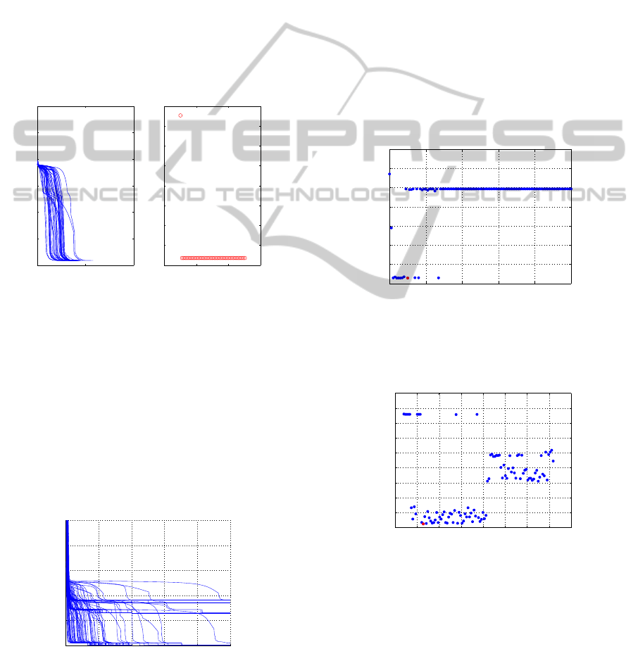
Using one of the MLPs(J=1), we employed SSF to
get MLP(J=2). Figure 4 shows how the learning went
on and the final MSEs. Most learnings stopped within
200 sweeps, and every learning reached the true opti-
mum, which is a wok-bottom since λ
max
/λ
min
≈ 10
4
.
As an existing method, we ran BPQ 100 times for
MLP (J=2). Figure 5 shows how each learning went
on and 70 runs reached the true optimum while the
others were trapped in the singular regions.
0 100 200 300 400 500
0
0.2
0.4
0.6
0.8
1
sweep
E
Figure 5: Learning process of an existing method for XOR
problem.
4.4 Experiment of Polynomial MLP
using Real Data
SSF was applied to ball bearings data (Journal of
Statistics Education) (N = 210). The objective is to
estimate fatigue (L10) using load (P), the number of
balls (Z), and diameter (D). Before learning, variables
were normalized as x
k
/max(x
k
) and (y − ¯y)/std(y).
We set as J
max
= 4.
In MLP(J=1) learning, we obtained three kinds of
solutions. For the next step of SSF we used the best
solution whose MSE is 0.2757.
SSF was applied to get MLP(J=2) from the
MLP(J=1) and the result is shown in Fig. 6. Most
final MSEs were located at 0.223 and 0.27. The
best MSE is 0.2229 and the solution is a gutter since
|λ
max
/λ
min
| ≈ 10
14
.
0 0.1 0.2 0.3 0.4 0.5
0.22
0.23
0.24
0.25
0.26
0.27
0.28
0.29
J =1−−>2,m =1
MSE
w
1
(2)
Figure 6: Result of SSF step from MLP(J=1) to MLP (J=2)
for ball bearings data.
3 4 5 6 7 8 9 10 11
0.185
0.19
0.195
0.2
0.205
0.21
0.215
0.22
0.225
0.23
J =2−−>3,m =1
MSE
w
1
(3)
Figure 7: Result of SSF step from MLP(J=2) to MLP (J=3)
for ball bearings data.
Then, SSF was applied to get MLP(J=3) from the
MLP(J=2) and the result is shown in Fig. 7. Final
MSEs were scattered in the form of three clusters.
The best MSE is 0.1862 and the solution is a gutter
since |λ
max
/λ
min
| ≈ 10
15
.
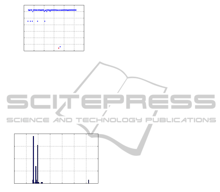
Finally, SSF was applied to get MLP(J=4) from
the MLP(J=3) and the result is shown in Fig. 8. Fi-
NCTA 2011 - International Conference on Neural Computation Theory and Applications
110
1 1.5 2 2.5 3 3.5 4
0.155
0.16
0.165
0.17
0.175
0.18
0.185
0.19
J =3−−>4,m =2
MSE
w
2
(4)
Figure 8: Result of SSF step from MLP(J=3) to MLP (J=4)
for ball bearings data.
nal MSEs were scattered in the form of three clusters.
The best MSE is 0.1571 and the solution is a gutter
since |λ
max
/λ
min
| ≈ 10
17
.
As an existing method, we ran BPQ 100 times for
MLP (J=4). Figure 9 shows the histogram of final
MSEs. The figure shows the MSE of the final SSF
solution is almost equivalent to that of the existing
method.
0 0.1 0.2 0.3 0.4 0.5 0.6
0
10
20
30
40
frequency
MSE
Figure 9: Solutions obtained by an existing method for ball
bearings data.
5 CONCLUSIONS
This paper proposed a new MLP learning called SSF,
which makes good use of singular regions. The
method begins with MLP(J=1) and gradually in-
creases the number of hidden units one by one. Our
various experiments showed that SSF found solutions
good enough for MLP(J). In the future we plan to
improve our method.
ACKNOWLEDGEMENTS
This work was supported by Grants-in-Aid for Sci-
entific Research (C) 22500212 and Chubu University
Grant 22IS27A.
REFERENCES
Amari, S. (1998). Natural gradient works efficiently in
learning. Neural Computation, 10(2):251–276.
Amari, S., Park, H. and Fukumizu, K. (2000). Adaptive
method of realizing natural gradient learning for mul-
tilayer perceptrons. Neural Computation, 12(6):1399–
1409.
Duda, R. O., Hart, P. E. and Stork, D. G. (2001). Pattern
classification, 2nd edition. John Wiley & Sons, Inc.
Fukumizu, K. and Amari,S.(2000). Local minima and
plateaus in heirarchical structure of multilayer percep-
trons. Neural Networks, 13(3):317–327.
Hamey, L. G. C. (1998). XOR has no local minima: a case
study in neural network error surface. Neural Net-
works, 11(4):669–681.
Minnett, R. C. J., Smith, A. T., Lennon Jr. W. C. and Hecht-
Nielsen, R. (2011). Neural network tomography: net-
work replication from output surface geometry. Neu-
ral Networks, 24(5):484–492.
Nakano, R. and Saito, K. (2002). Discovering polynomials
to fit multivariate data having numeric and nominal
variables. LNAI 2281:482–493.
Watanabe, S. (2009). Algebraic geometry and statistical
learning theory. Cambridge Univ. Press.
Saito, K. and Nakano, R. (1997). Partial BFGS update and
efficient step-length calculation for three-layer neural
networks. Neural Computation, 9(1):239–257.
Sussman, H. J. (1992). Uniqueness of the weights for min-
imal feedforward nets with a given input-output map.
Neural Networks, 5(4):589–593.
LEARNING METHOD UTILIZING SINGULAR REGION OF MULTILAYER PERCEPTRON
111
