
A COMPARATIVE EVALUATION OF PROXIMITY MEASURES FOR
SPECTRAL CLUSTERING
Nadia Farhanaz Azam and Herna L. Viktor
School of Electrical Engineering and Computer Science, University of Ottawa
800 King Edward Avenue, Ottawa, Ontario K1N6N5, Canada
Keywords:
Spectral clustering, Proximity measures, Similarity measures, Boundary detection.
Abstract:
A cluster analysis algorithm is considered successful when the data is clustered into meaningful groups so that
the objects in the same group are similar, and the objects residing in two different groups are different from
one another. One such cluster analysis algorithm, the spectral clustering algorithm, has been deployed across
numerous domains ranging from image processing to clustering protein sequences with a wide range of data
types. The input, in this case, is a similarity matrix, constructed from the pair-wise similarity between the data
objects. The pair-wise similarity between the objects is calculated by employing a proximity (similarity, dis-
similarity or distance) measure. It follows that the success of a spectral clustering algorithm therefore heavily
depends on the selection of the proximity measure. While, the majority of prior research on the spectral clus-
tering algorithm emphasizes the algorithm-specific issues, little research has been performed on the evaluation
of the performance of the proximity measures. To this end, we perform a comparative and exploratory anal-
ysis on several existing proximity measures to evaluate their suitability for the spectral clustering algorithm.
Our results indicate that the commonly used Euclidean distance measure may not always be a good choice
especially in domains where the data is highly imbalanced and the correct clustering of the boundary objects
are crucial. Furthermore, for numeric data, measures based on the relative distances often yield better results
than measures based on the absolute distances, specifically when aiming to cluster boundary objects. When
considering mixed data, the measure for numeric data has the highest impact on the final outcome and, again,
the use of the Euclidian measure may be inappropriate.
1 INTRODUCTION
In recent years, a new family of cluster analysis algo-
rithms, collectively known as the Spectral Clustering
algorithms, has gained much interest in the research
community. One of the main strengths of the spectral
clustering algorithm is that the algorithm may be ap-
plied to a wide range of data types (i.e. numeric, cate-
gorical, binary, and mixed) as they are not sensitive to
any particular data type. These algorithms consider
the pair-wise similarity between the data objects to
construct a similarity (also known as proximity, affin-
ity, or weight) matrix. The eigenvectors and eigen-
values of this similarity matrix are then used to find
the clusters ((Luxburg, 2007), (Shi and Malik, 2000),
(Ng et al., 2001)). The various algorithms from this
family mainly differ with respect to how the similarity
matrix is manipulated and/or which eigenvalue(s) and
eigenvector(s) are used to partition the objects into
disjoint clusters. Significant theoretical progress has
been made regarding the improvement of the spectral
clustering algorithms as well as the proposal of new
methods, or the application in various domains such
as image segmentation and speech separation. How-
ever, little research has been performed on the selec-
tion of proximity measures, which is a crucial step in
constructing the similarity matrix. In this paper, we
evaluate the performance of a number of such prox-
imity measures and perform an explorative study on
their behavior when applied to the spectral clustering
algorithms.
Proximity measures, i.e. similarity, dissimilar-
ity and distance measures, often play a fundamen-
tal role in cluster analysis (Jain et al., 1999). Early
steps of the majority of cluster analysis algorithms of-
ten require the selection of a proximity measure and
the construction of a similarity matrix (if necessary).
Most of the time, the similarity matrix is constructed
from an existing similarity or distance measure, or by
introducing a new measure specifically suitable for
a particular domain or task. It follows that the se-
lection of such measures, particularly when existing
30
Farhanaz Azam N. and Viktor H..
A COMPARATIVE EVALUATION OF PROXIMITY MEASURES FOR SPECTRAL CLUSTERING.
DOI: 10.5220/0003649000300041
In Proceedings of the International Conference on Knowledge Discovery and Information Retrieval (KDIR-2011), pages 30-41
ISBN: 978-989-8425-79-9
Copyright
c
2011 SCITEPRESS (Science and Technology Publications, Lda.)

measures are applied, requires careful consideration
as the success of these algorithms relies heavily on the
choice of the proximity function ((Luxburg, 2007),
(Bach and Jordan, 2003), (Everitt, 1980)).
Most of the previous studies on the spectral clus-
tering algorithm use the Euclidean distance mea-
sure, a distance measure based on linear differences,
to construct the similarity matrix for numeric fea-
ture type ((Shi and Malik, 2000), (Ng et al., 2001),
(Verma and Meila, 2001)) without explicitly stating
the consequences of selecting the distance measure.
However, there are several different proximity mea-
sures available for numeric variable types. Each of
them has their own strengths and weaknesses. To
our knowledge, no in-depth evaluation of the perfor-
mance of these proximity measures on spectral clus-
tering algorithms, specifically showing that the Eu-
clidean distance measure outperforms, has been car-
ried out. As such, an evaluation and an exploratory
study that compares and analyzes the performance of
various proximity measures may potentially provide
important guideline for researchers when selecting a
proximity measure for future studies in this area. This
paper endeavors to evaluate and compare the perfor-
mance of these measures and to imply the conditions
under which these measures may be expected to per-
form well.
This paper is organized as follows. In Section 2,
we discuss the two spectral clustering algorithms that
we used in our experiment. Section 3 presents an
overview of several proximity measures for numeric,
and mixed variable types. This is followed by Section
4, where we present our experimental approach and
evaluate and analyze the results obtained from our ex-
periments. We conclude the paper in Section 5.
2 SPECTRAL CLUSTERING
Spectral clustering algorithms originated from the
area of graph partitioning and manipulate the eigen-
value(s) and eigenvector(s) of the similarity matrix to
find the clusters. There are several advantages, when
compared to other cluster analysis methods, to ap-
plying the spectral clustering algorithms ((Luxburg,
2007), (Ng et al., 2001), (Aiello et al., 2007), (Fis-
cher and Poland, 2004)). Firstly, the algorithms do
not make assumption on the shape of the clusters. As
such, while spectral clustering algorithms may be able
to find meaningful clusters with strongly coherent ob-
jects, algorithms such as K-means or K-medians may
fail to do so. Secondly, the algorithms do not suffer
from local minima. Therefore, it may not be neces-
sary to restart the algorithm with various initialization
options. Thirdly, the algorithms are also more stable
than some algorithms in terms of initializing the user-
specific parameters (i.e. the number of clusters). As
such, the user-specific parameters may often be esti-
mated accurately with the help of theories related to
the algorithms. Prior studies also show that the al-
gorithms from this group thus often outperform tra-
ditional clustering algorithms, such as, K-means and
Single Linkage (Luxburg, 2007). Importantly, the al-
gorithms from the spectral family are able to handle
different types of data (i.e. numeric, nominal, binary,
or mixed) and one only needs to convert the dataset
into a similarity matrix to be able to apply this algo-
rithm on a given dataset (Luxburg, 2007).
The spectral clustering algorithms are divided into
two types, namely recursive algorithms and multi-
way algorithms (Verma and Meila, 2001). In this
paper, we consider two algorithms, one from each
group. From the first group, we select the normal-
ized cut spectral clustering algorithm as this algorithm
proved to have had several practical successes in a va-
riety of fields (Shi and Malik, 2000). We refer to this
algorithm as SM (NCut) in the remainder of the pa-
per. The Ng, Jordan and Weiss algorithm is an im-
provement to the algorithm proposed by Meila and
Shi(Meila and Shi, 2001) and therefore, we select this
algorithm (refer to as NJW(K-means)) from the sec-
ond group. In the following section we present several
algorithm-specific notations before we discuss the al-
gorithms themselves.
2.1 Notations
Similarity Matrix or Weight Matrix, W . Let W
be an N × N symmetric, non-negative matrix where
N is the number of objects in a given dataset. Let i
and j be any two objects in a given dataset, located
at row i and row j, respectively. If the similarity (i.e.
calculated from a proximity measure) between these
two objects is w
i, j
, then it will be located at the cell at
row i and column j in the weight matrix.
Degree Matrix, D. Let d be an N × 1 matrix with
d
i
=
∑
n
j=1
w
i, j
as the entries which denote the total
similarity value from object i to the rest of the objects.
Therefore, the degree matrix D is an N × N diagonal
matrix which contains the elements of d on its main
diagonal.
Laplacian Matrix, L. The Laplacian matrix is con-
structed from the weight matrix W and the degree ma-
trix D. The main diagonal of this matrix is always
non-negative. In graph theory, the eigenvector(s) and
eigenvalue(s) of this matrix contain important infor-
A COMPARATIVE EVALUATION OF PROXIMITY MEASURES FOR SPECTRAL CLUSTERING
31

mation about the underlying partitions present in the
graph. The spectral clustering algorithms also use
the same properties to find the clusters from a given
dataset.
2.2 The SM (NCut) Algorithm
The SM (NCut) spectral clustering algorithm (Shi and
Malik, 2000) is one of the most widely used recur-
sive spectral clustering algorithm ((Luxburg, 2007),
(Verma and Meila, 2001)). The main intuition behind
this algorithm is the optimization of an objective func-
tion called the Normalized Cut, or NCut. Minimizing
the NCut function is the same as finding a cut such
that the total connection in between two groups is
weak, whereas the total connection within each group
is strong. The algorithm uses the eigenvector associ-
ated with the second smallest eigenvalue of the gen-
eralized eigenvalue system which is considered as the
real valued solution to the Normalized Cut problem.
The partitions are obtained by thresholding this eigen-
vector. There are a number of ways this grouping may
be performed. One may use a particular point (i.e.
zero, mean, median) as the splitting criteria or use an
existing algorithm such as the K-means or K-medians
algorithms for this purpose. Components with simi-
lar values usually reside in the same cluster. Since,
this algorithm bi-partition the data, we get two dis-
joint clusters. To find more clusters we need to re-
partition the segments by recursively applying the al-
gorithm on each of the partitions.
2.3 The NJW (K-means) Algorithm
In contrast to the SM (NCut) algorithm that min-
imizes the NCut objective function and recursively
bi-partitions the data, this algorithm directly parti-
tions the data into k groups. The algorithm manip-
ulates the normalized Laplacian matrix to find the
clusters. The algorithm relates various theories from
the Random Walk Problem and Matrix Perturbation
Theory to theoretically motivate the partitioning solu-
tion ((Luxburg, 2007), (Ng et al., 2001), (Meila and
Shi, 2001)). Once the eigensystem is solved and the
k largest eigenvectors are normalized, the algorithm
uses the K-means algorithm to find the k partitions.
3 PROXIMITY MEASURES
Proximity measures quantify the distance or close-
ness between two data objects. They may be sub-
categorized into three types of measures, namely sim-
ilarity, dissimilarity, and distance.
Similarity is a numerical measure that represents
the similarity (i.e. how alike the objects are) between
two objects. This measure usually returns a non-
negative value that falls in between 0 and 1. How-
ever, in some cases similarity may also range from −1
to +1. When the similarity takes a value 0, it means
that there is no similarity between the objects and the
objects are very different from one another. In con-
trast, 1 denotes complete similarity, emphasizing that
the objects are identical and possess the same attribute
values.
The dissimilarity measure is also a numerical
measure, which represents the discrepancy or the dif-
ference between a pair of objects (Webb, 2002). If
two objects are very similar then the dissimilarity
measure will have a lower value, and visa versa.
Therefore, this measure is reversely related to the sim-
ilarity measure. The dissimilarity value also usually
fall into the interval [0, 1], but it may also take values
ranging from −1 to +1.
The term distance, which is also commonly used
as a synonym for the dissimilarity measure, com-
putes the distance between two data points in a multi-
dimensional space. Let d(x,y) be the distance be-
tween objects x and y. Then, the following four prop-
erties hold for a distance measure ((Larose, 2004),
(Han and Kamber, 2006)):
1. d(x,y) = d(y,x), for all points x and y.
2. d(x,y) = 0, if x = y.
3. d(x,y) ≥ 0, for all points x and y.
4. d(x,y) ≤ d(x, z) + d(z, y), for all points x, y and
z. This implies that introducing a third point
may never shorten the distance between two other
points.
There are many different proximity measures
available in the literature. One of the reasons for this
variety is that these measures differ on the data type
of the objects in a given dataset. Next we present the
proximity measures that are used in this paper.
3.1 Proximity Measures for Numeric
Variables
Table 1 presents the measures for numeric, real-
valued or continuous variables used in our paper
((Webb, 2002), (Teknomo, 2007)). These measures
may be categorized into three groups. The first group
contains the functions that measure the absolute dis-
tance between the objects and are scale dependent.
This list includes the Euclidean (EUC), Manhattan
(MAN), Minkowski (MIN), and Chebyshev (CHEB)
distances. The second group contains only the Can-
KDIR 2011 - International Conference on Knowledge Discovery and Information Retrieval
32

Table 1: Proximity measures for numeric variables.
Name Function Discussion
Euclidean
Distance (EUC)
d
x
i
,x
j
=
q
∑
n
k=1
(x
ik
− x
jk
)
2
Works well for compact or isolated clusters; Discovers clusters of spher-
ical shape; Any two objects may not be influenced by the addition of
a new object (i.e. outliers); Very sensitive to the scales of the vari-
ables; Not suitable for clusters of different shapes; The variables with
the largest values may always dominate the distance.
Manhattan Dis-
tance (MAN)
d
x
i
,x
j
=
∑
n
k=1
|x
ik
− x
jk
| Computationally cheaper than the Euclidean distance; Scale dependent.
Minkowski Dis-
tance (MIN)
d
x
i
,x
j
=
∑
n
k=1
|x
ik
− x
jk
|
λ
1
λ
One may control the amount of emphasis given on the larger differ-
ences; The Minkowski distance may cost more than the Euclidean and
Manhattan distance when λ > 2.
Chebyshev Dis-
tance (CHEB)
d
x
i
,x
j
= max
k
|x
ik
− x
jk
| Suitable for situations where the computation time is very crucial; Very
sensitive to the scale of the variables.
Canberra Dis-
tance (CAN)
d
x
i
,x
j
=
∑
n
k=1
|x
ik
−x
jk
|
|x
ik
+x
jk
|
Not scale sensitive; Suitable for non-negative values; Very sensitive to
the changes near the origin; Undefined when both the coordinates are 0.
Mahalanobis
Distance
(MAH)
d(~x,~y) =
p
(~x −~y)C
−1
(~x −~y)
T
Considers the correlation between the variables; Not scale dependent;
Favors the clusters of hyper ellipsoidal shape; Computational cost is
high; May not be suitable for high-dimensional datasets.
Angular Dis-
tance (COS)
d
x
i
,x
j
= 1 −
∑
n
k=1
x
ik
·x
jk
(
∑
n
k=1
x
2
ik
·
∑
n
k=1
x
2
jk
)
1
2
Calculates the relative distance between the objects from the origin;
Suitable for semi-structured datasets (i.e. Widely applied in Text Doc-
ument cluster analysis where data is highly dimensional); Does not de-
pend on the vector length; Scale invariant; Absolute distance between
the data objects is not captured.
Pearson Corre-
lation Distance
(COR)
d
i j
= 1−
∑
n
k=1
(x
ik
− ¯x
i
)·(x
jk
− ¯x
j
)
(
∑
n
k=1
(x
ik
− ¯x
i
)
2
·
∑
n
k=1
(x
jk
− ¯x
j
)
2
)
1
2
Scale invariant; Considers the correlation between the variables; Cal-
culates the relative distance between the objects from the mean of the
data; Suitable for semi-structured data analysis (i.e. applied in microar-
ray analysis, document cluster analysis); Outliers may affect the results.
berra distance (CAN) which also calculates the abso-
lute distance, however, the measure is not scale de-
pendent. In the third group we have three distance
measures, namely the Angular or Cosine (COS), Pear-
son Correlation (COR), and Mahalanobis (MAH) dis-
tances. These measures consider the correlation be-
tween the variables into account and are scale invari-
ant.
3.2 Proximity Measures for mixed
Variables
In the previous section, we concentrated our discus-
sion on datasets with numeric values. Nevertheless,
in practical applications, it is often possible to have
more than one type of attribute in the same dataset. It
follows that, in such cases, the conventional proximity
measures for those data types may not work well. A
more practical approach is to process all the variables
of different types together and then perform a sin-
gle cluster analysis (Kaufman and Rousseeuw, 2005).
The Gower’s General Coefficient and Laflin’s General
Coefficient are two such functions that incorporate in-
formation from various data types into a single simi-
larity coefficient. Table 2 provides the equations and
additional information about these two coefficients.
4 EXPERIMENTS
This section discusses our experimental methodology
and the results obtained for each of the data types.
In order to compare the performance of the proximity
measures for a particular data type, we performed ten-
fold cross validation (Costa et al., 2002) and classes
to clusters evaluation on each of the datasets. In
this paper, we consider the external measures when
evaluating our results, as the external class labels for
each of the datasets used were available to us. More-
over, this allows us to perform a fair comparison
against the known true clusters for all the proximity
measures. We used two such measures namely, F-
measure ((Paccanaro et al., 2006), (Steinbach et al.,
2000)) and G-means (Kubat et al., 1998). In addi-
tion, we used the Friedman Test (Japkowicz and Shah,
2011) to test the statistical significance of our results.
The test is best suited for situations, like ours, where
multiple comparisons are performed against multiple
datasets. It returns the p-value that helps us to deter-
mine whether to accept or reject the null hypothesis.
For us the null hypothesis was “the performance of
all the proximity measure is equivalent”. For exam-
ple, a p-value less than 0.05 signify that the result is
only 5% likely to be extraordinary ((Japkowicz and
Shah, 2011), (Boslaugh and Watters, 2008)).
A COMPARATIVE EVALUATION OF PROXIMITY MEASURES FOR SPECTRAL CLUSTERING
33

Table 2: Proximity measures for mixed variables.
Name Function Discussion
Gower’s General Coeffi-
cient (GOWER)
d(i, j) =
∑
p
f =1
δ
( f )
i j
d
( f )
i j
∑
p
f =1
δ
( f )
i j
For this coefficient δ
( f )
i j
= 0, if one of the values is missing or
the variable is of type asymmetric binary variable. Otherwise,
δ
( f )
i j
= 1. For numeric variables distance is calculated using the
formula: d
( f )
i j
=
|x
i f
−x
j f
|
max
h
x
h f
−min
h
x
h f
. For binary and nominal variables
the dissimilarity is the number of un matched pairs. This measure
may be extended to incorporate other attribute types (e.g. ordinal,
ratio-scaled) (Han and Kamber, 2006).
Laflin’s General Similar-
ity Coefficient (LAFLIN)
s(i, j) =
N
1
.s
1
+N
2
.s
2
+...+N
n
.s
n
N
1
+N
2
+...+N
n
In this function, N
1
...N
n
represent the total number of attributes
of each of the variable type, whereas, s
1
...s
n
represent the total
similarity measure calculated for each of the attribute type. The
function uses existing similarity measures to calculate the similar-
ity scores s
1
...s
n
.
Table 3: Dataset Information.
Numeric Datasets
Dataset No. of No. of True No. of
Tuples Clusters Attributes
Body 507 2 21
Iris 150 3 4
Wine 178 3 13
Glass 214 6 8
Ecoli 336 5 7
SPECT 267 2 44
Mixed Datasets
Dataset No. of No. of True No. of
Tuples Clusters Attributes
Automobile 205 6 25
CRX 690 2 15
Dermatology 366 6 33
Hepatitis 155 2 19
Post-Operative 90 3 8
Soybean 290 15 35
4.1 Implementation and Settings
For all the experiments in this paper, the data prepro-
cessing (e.g. replacing missing values, standardiza-
tion) was performed using WEKA (Witten and Frank,
2005), an open-source Java-based machine learning
software, developed at the University of Waikato
in New Zealand. The spectral cluster analysis al-
gorithms are implemented in MATLAB
R
. Since
these algorithms manipulate the similarity matrix of
a dataset, computation of eigenvalues and eigenvec-
tors of the similarity matrix may be inefficient for a
large matrix. However, MATLAB efficiently solves
the eigensystem of large matrices. The cluster evalu-
ation measures have been implemented in Java.
4.2 Datasets
Six datasets are used for each of the data types. All
the datasets varied in size and are based on real-world
problems representing various domains and areas. As
for numeric data type, several proximity measures are
scale-dependent. As such, we standardized (Han and
Kamber, 2006) the attribute values to ensure the ac-
curacy of our results. In addition, we used Equation 1
to convert the distance measure into a similarity mea-
sure in order to create the similarity or weight matrix
W (Shi and Malik, 2000). It is also important to note
that the selection of sigma is very crucial to the suc-
cess of spectral clustering algorithm and the value of
sigma varies depending on the proximity measure and
the dataset used. We adopted the method proposed by
Shi and Malik in (Shi and Malik, 2000) to select the
sigma value. The sigma returned through this method
was used as a starting point. Each of our experiments
were performed on a range of values surrounding that
sigma value and the result for which we achieved the
best scores are included in this paper.
s(x,y) = exp(
−d(x, y)
2
2 × σ
2
) (1)
Five of our datasets are from UCI repository (Asun-
cion and Newman, 2007) and one of them (Body
dataset) is from an external source (Heinz et al.,
2003). In Table 3, we provide a summary of the nu-
meric datasets. The six datasets used for the mixed
variable type are also obtained from the UCI reposi-
tory. A summary of the mixed datasets is presented in
Table 3.
4.3 Experimental Results for Numeric
Datasets
In Table 4 and Table 5 we present the F-measure and
G-means scores obtained for the datasets with nu-
meric variables when SM (NCut) algorithm is used.
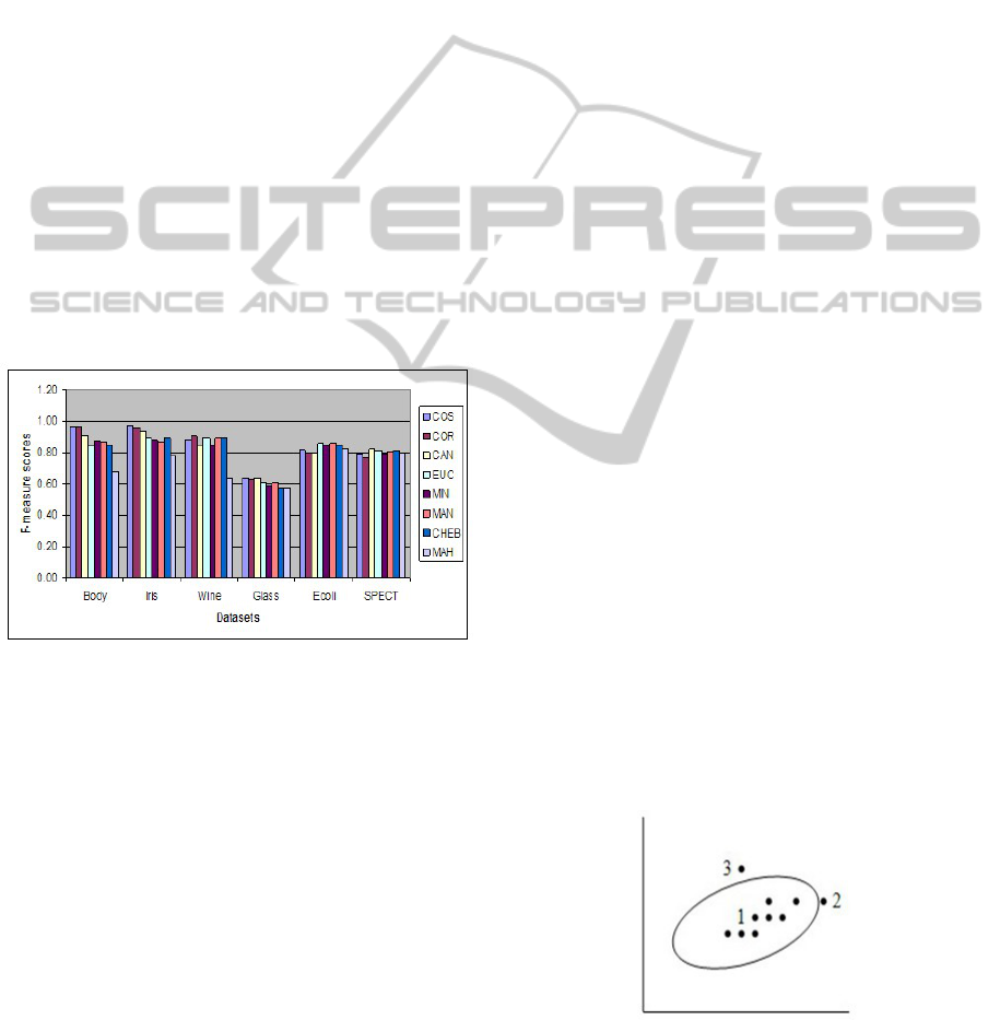
Our results show that the COR distance and the COS
distance measure often scored higher than the rest of
the distance measures (Figure 1). These two distance
measures performed well in four out of six datasets.
The datasets are Body, Iris, Wine, and Glass. We also
notice that most of the time, these two coefficients
KDIR 2011 - International Conference on Knowledge Discovery and Information Retrieval
34
achieved similar values for both the evaluation mea-
sures. The overall average difference for these two
distance measures is 0.02, irrespective of the dataset
or the splitting method used. In contrast, the MAH
distance measure performed poorly in four out of six
datasets. The datasets for which this distance measure
scored the lowest are Body, Iris, Wine, and Glass. The
MAN distance performed well for the Ecoli dataset
and the CAN distance performed best for the SPECT
dataset. We also notice that the performances of EUC,
MIN, MAN, CAN and CHEB distances are very sim-
ilar, and that they often scored moderately, in com-
parison to the highest and the lowest scores. For
example, based on the scores obtained for the Body
dataset, the distance measures may be grouped into
three groups: 1) the COS distance and COR distance
measure in one group where the scores fall in the
range [0.96 − 0.97], 2) the CAN, EUC, MIN, MAN
and CHEB distance measures in the second group
where the range is [0.85 − 0.90], and 3) the MAH dis-
tance measure which scores the lowest (0.68). As ob-
served from the results, the EUC distance measure,
which is often used in the spectral cluster analysis al-
gorithms, may not always be a suitable choice.
Figure 1: F-measure scores for the numeric dataset when
tested on the SM (NCut) algorithm.
We observe that, if the COS distance or the COR
distance measure is used instead of the EUC distance,
on average the performance improved by 7.42% (F-
measure) and 8.17% (G-means), respectively, for our
datasets. In Table 6 and Table 7, we provide the eval-
uation scores from the NJW (K-means) algorithm. In
this case also, the results showed almost the same
trend as the results from the SM (NCut) algorithm.
For both the evaluation measures, the results indicate
that the MAH distance measure often scored the low-
est scores over a range of datasets. Among the six
datasets, in five of the cases the MAH distance scored
the lowest scores. These datasets are: Body, Iris,
Wine, Glass, and Ecoli. Furthermore, in none of the
cases, the EUC distance measure scored the highest
score. For two datasets (i.e. Body and Iris), the COR
distance and the COS distance performed well, and
for the Wine and Glass datasets, the scores were very
close to the highest scores achieved. The MAN dis-
tance performed well for the Ecoli and Glass datasets.
The Friedman Test which was used to measure the
statistical significance of our results, gives p-values of
0.0332 (SM (NCut)) and 0.0097 (NJW (K-means)),
respectively. Since the p-values are less than 0.05,
this indicates the results are statistically significant.
Our results showed that the MAH distance often per-
formed poorly when compared to the rest of the dis-
tance measures according to the cluster evaluation
measures. We noticed that, when the MAH distance is
used, the spectral clustering algorithms produced im-
balanced clusters. Here the clusters are imbalanced
when one partition contains relatively fewer objects
than the other cluster. We also noticed that the objects
that are placed in the smaller cluster are the objects
that have the lowest degree. Recall from Section 2
that the degree is the total similarity value from one
object to the rest of the objects in a dataset. In spec-
tral clustering, the objects are considered as nodes in
the graph, and a partition separates objects where the
total within cluster similarity is high and the between
cluster similarity is very low. Therefore, when the
degree is low for an object, compared to the rest of
the objects, it indicates that the object is less simi-
lar than most of the objects in the dataset. Now, the
equation of the MAH distance defines an ellipsoid in
n-dimensional space ((Lee and Verri, 2002), (Abou-
Moustafa and Ferrie, 2007)). The distance considers
the variance (how spread out the values are from the
mean) of each attribute as well as the covariance (how
much two variables change together) of the attributes
in the datasets. It gives less weight to the dimensions
with high variance and more weight to the dimen-
sions with small variance. The covariance between
the attributes allows the ellipsoid to rotate its axes
and increase and decrease its size (Abou-Moustafa
and Ferrie, 2007). Therefore, the distance measure is
very sensitive to the extreme points (Filzmoser et al.,
2005).
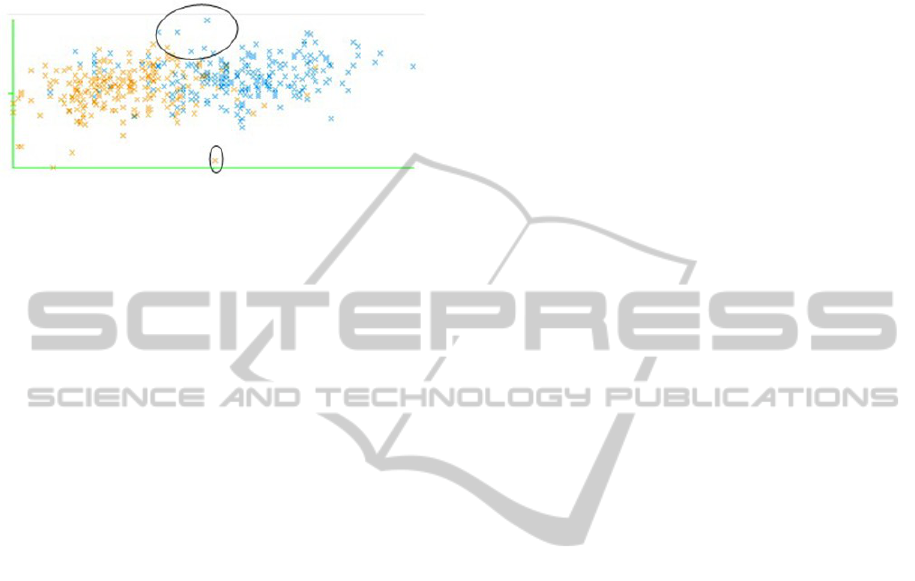
Figure 2: A scenario depicting the Mahalanobis (MAH) dis-
tance between three points.
Figure 2 illustrates a scenario showing the MAH
A COMPARATIVE EVALUATION OF PROXIMITY MEASURES FOR SPECTRAL CLUSTERING
35

Table 4: F-measure scores for Numeric datasets. Algorithm: SM (NCut), Splitting points: Zero and Mean value respectively.
Dataset COS COR CAN EUC MIN MAN CHEB MAH
Body 0.97 0.96 0.90 0.87 0.87 0.87 0.85 0.68
0.97 0.96 0.90 0.84 0.87 0.87 0.85 0.68
Iris 0.97 0.96 0.94 0.90 0.88 0.86 0.88 0.79
0.97 0.96 0.94 0.89 0.88 0.86 0.89 0.78
Wine 0.91 0.95 0.84 0.81 0.84 0.90 0.87 0.79
0.88 0.90 0.85 0.89 0.85 0.89 0.89 0.64
Glass 0.62 0.61 0.61 0.61 0.60 0.61 0.59 0.60
0.64 0.63 0.64 0.61 0.59 0.61 0.57 0.57
Ecoli 0.81 0.79 0.83 0.82 0.83 0.85 0.82 0.81
0.81 0.80 0.80 0.86 0.85 0.86 0.85 0.82
SPECT 0.80 0.77 0.81 0.80 0.80 0.81 0.80 0.80
0.79 0.77 0.82 0.81 0.79 0.81 0.81 0.80
Table 5: G-means scores for Numeric datasets. Algorithm: SM (NCut), Splitting points: Zero and Mean value respectively.
Dataset COS COR CAN EUC MIN MAN CHEB MAH
Body 0.97 0.96 0.90 0.87 0.87 0.87 0.85 0.71
0.97 0.97 0.90 0.83 0.84 0.87 0.85 0.71
Iris 0.97 0.96 0.94 0.90 0.88 0.87 0.88 0.80
0.97 0.96 0.94 0.90 0.89 0.87 0.89 0.80
Wine 0.92 0.95 0.86 0.83 0.86 0.91 0.87 0.80
0.89 0.91 0.86 0.90 0.86 0.90 0.89 0.67
Glass 0.65 0.64 0.65 0.66 0.64 0.64 0.64 0.62
0.66 0.65 0.67 0.64 0.62 0.64 0.61 0.60
Ecoli 0.82 0.80 0.83 0.82 0.83 0.86 0.83 0.81
0.81 0.81 0.81 0.86 0.86 0.86 0.85 0.82
SPECT 0.81 0.80 0.82 0.82 0.81 0.81 0.80 0.82
0.81 0.80 0.83 0.82 0.82 0.82 0.81 0.81
Table 6: F-measure scores of the NJW (K-means) algorithm (tested on numeric dataset).
Dataset COS COR CAN EUC MIN MAN CHEB MAH
Body 0.88 0.88 0.83 0.79 0.79 0.80 0.78 0.64
Iris 0.81 0.82 0.79 0.78 0.80 0.78 0.79 0.69
Wine 0.94 0.96 0.97 0.85 0.97 0.86 0.83 0.50
Glass 0.54 0.54 0.53 0.55 0.56 0.58 0.54 0.50
Ecoli 0.65 0.72 0.63 0.74 0.73 0.75 0.65 0.48
SPECT 0.77 0.77 0.77 0.77 0.77 0.77 0.76 0.77
Table 7: G-means scores of the NJW (K-means) algorithm (tested on numeric dataset).
Dataset COS COR CAN EUC MIN MAN CHEB MAH
Body 0.88 0.88 0.83 0.79 0.79 0.80 0.78 0.67
Iris 0.81 0.83 0.79 0.79 0.80 0.79 0.79 0.69
Wine 0.94 0.96 0.97 0.86 0.97 0.87 0.84 0.57
Glass 0.56 0.55 0.56 0.58 0.58 0.62 0.56 0.55
Ecoli 0.69 0.74 0.68 0.75 0.75 0.77 0.68 0.52
SPECT 0.80 0.80 0.80 0.80 0.80 0.80 0.79 0.80
distance between the objects. In this figure, the dis-
tance between object 1 and 2 will be less than the dis-
tance between object 1 and 3, according to the MAH
distance. This is because, object 2 lies very close to
the main axes along with the other objects, whereas
the object 3 lies further away from the main axes.
Therefore, in such situations, the MAH distance will
be large. For numeric data, the similarity will be very
low when the distance is very large. The function in
Equation 1, which is used to convert a distance value
into a similarity value, will give a value close to zero
when the distance is very large. Therefore, the de-
gree from this object to the remainder of the objects
becomes very low and the spectral methods separate
these objects from the rest. This is one of the possible
reasons for the MAH distance performing poorly. It
either discovers imbalanced clusters or places similar
objects wrongly into two different clusters. Conse-
KDIR 2011 - International Conference on Knowledge Discovery and Information Retrieval
36
quently, one possible way to improve the performance
of the MAH distance measure might be by changing
the value of σ to a larger value. In this way, we may
prevent the similarity to have a very small value.
Figure 3: Example of cluster assignments of the Body
dataset. The circles are used to point to the several indi-
vidual members that are placed differently.
Our results also indicate that the COR and COS
distances performed best for four out of six datasets.
Both of the distance measures calculate the relative
distance from a fixed point (mean or zero, respec-
tively). Therefore, two objects with a similar pat-
tern will be more similar even if their sizes are differ-
ent. The EUC, MAN, MIN, CAN and CHEB distance
measures, however, calculate the absolute distance
(i.e. straight line distance from one point to another).
For instance, the Body dataset partitions the objects
into two main clusters, one with larger body dimen-
sions and another cluster with smaller body dimen-
sions. According to the true cluster information, the
larger body dimensions denote the Male population
and the smaller body dimensions denote the Female
population. When compared to the true clusters, we
observed that several individuals, whose body dimen-
sions are comparatively lower than the average body
dimensions of the Male population, are placed with
the individuals from the Female population by the dis-
tance measures that calculate the absolute distance.
Conversely, Female individuals with larger body di-
mensions than the average body dimensions of the Fe-
male population are placed with the individuals from
Male population. Therefore, these individuals that fall
very close to the boundary of the two true clusters,
are placed differently by the distance measures that
calculate the absolute distance (i.e. EUC distance,
MAN distance, and MIN distance) than the distance
measures that consider the relative distance (i.e. COR
distance and COS distance). In such cases, the COS
distance and the COR distance correctly identify these
individuals. In Figure 3 we plot the first two attributes
of the Body dataset when the EUC distance is used
as the distance measure. The object marked with a
smaller circle is an example of a Male individual with
smaller body dimensions. When the EUC distance is
used as the distance measure in the spectral cluster-
ing algorithm, this object is placed with the Female
population. The objects marked with the larger circle
illustrate the reversed situation, where Female indi-
viduals with larger body size are placed with the in-
dividuals from Male population. In both situations,
the COR and COS distances placed the objects within
their own groups. In Figure 4, we provide the clus-
ters from the Ecoli dataset when the MAN (Left) and
the COS (Middle) distances are used. The farthest
right figure (with the title Original) depicts the true
clusters. The objects, according to the true clusters,
overlap between the clusters in a number of situations
(e.g. the objects marked with circle 2 and 4, or the
objects marked with circle 3 and 5). This indicates
that there are several objects in the dataset that may
be very similar, but are placed in two different true
clusters. When the spectral clustering algorithms are
applied to this dataset, both the COS and MAN dis-
tances divide the true cluster marked with circle 1 (in
Figure 4) into two different clusters. However, the
clusters produced by the COS distance contain mem-
bers from true cluster 1 and 3, whereas the clusters
produced by the MAN distance contain the members
from true cluster 1. The figure indicates that the shape
of the clusters produced by the COS distance are more
elongated toward the origin, which is the reason why
some of the members from true cluster 3 are included.
4.3.1 Discussion
The main conclusion drawn from our results thus in-
dicate that the MAH distance needs special considera-
tion. This measure tends to create imbalanced clusters
and therefore results in poor performance. In addi-
tion, the distance measures based on the relative dis-
tances (i.e. COR and COS distance measure) outper-
formed the distance measures based on the absolute
distance. We noticed that, in such cases, the objects
that reside in the boundary area are correctly identi-
fied by the relative distance measures. These bound-
ary objects are slightly different from the other mem-
bers of their own group and may need special atten-
tion. This is due to the fact that the COR and COS
measures consider the underlying patterns in between
the objects from a fixed point (i.e. mean or zero), in
contrast to the absolute distance approaches. There-
fore, the Euclidian (EUC) distance which is a com-
monly used absolute distance measure in clustering
domains, may not always be a good selection for the
spectral clustering algorithm, especially in domains
where we are sensitive to outliers and anomalies.
A COMPARATIVE EVALUATION OF PROXIMITY MEASURES FOR SPECTRAL CLUSTERING
37
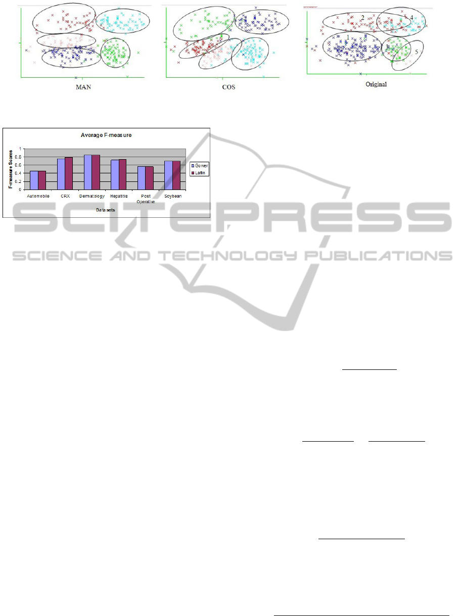
Figure 4: Example of cluster assignments of the Ecoli dataset. (Left) The clusters obtained by using the MAN distance
measure, (Middle) the clusters obtained by using the COS distance, and (Right) the original true clusters.
Figure 5: Average F-measure scores for the Mixed Datasets
when tested on the SM(NCut) algorithm.
4.4 Experimental Results for mixed
Datasets
In Table 8, we present the F-measure and G-means
scores for the Mixed datasets, when tests are applied
on the SM (NCut) algorithm. The results from NJW
(K-means) algorithm are given in Table 9. Figure 5
presents a graphical representation of our results. Our
results from the external evaluation scores show that,
the GOWER coefficient performed well for the Auto-
mobile and Dermatology dataset. The LAFLIN’s co-
efficient also performed well for two of the datasets.
The datasets are CRX and Hepatitis. For Post Opera-
tive and Soybean datasets, both the coefficients scored
the same scores. In contrast, when the tests are ap-
plied on the NJW (K-means) algorithm, our results in-
dicate that the GOWER coefficient performed slightly
better than the LAFLIN’s. In four out of six datasets
the GOWER scored slightly higher scores than the
LAFLIN’s coefficient. The datasets are Automobile,
Dermatology, Post Operative, and Soybean. For this
case also, the LAFLIN’s coefficient performed best
for the same two datasets (i.e. CRX and Hepatitis) as
our previous test on the SM (NCut) algorithm. How-
ever, we also noticed from the scores that the differ-
ence between the performances of the two coefficients
is very low. The p-values from the Friedman test are
0.3173 and 0.4142, respectively. Since, both the val-
ues are greater than 0.05, the difference between the
performance of the two coefficients is not statistically
significant.
In this part, we analyze the coefficients to deter-
mine the relationship between them. The equations
for the two coefficients are given in Table 2. For the
GOWER coefficient, the term δ
( f )
i j
is an indicator vari-
able associated with each of the variables present in
the dataset and the term d
( f )
i j
is the distance or dissim-
ilarity calculated for each variable for objects i and j.
We also know from the description given in Table 2
that δ
( f )
i j
= 0 for the asymmetric binary variables and
for all the other types δ
( f )
i j
= 1. In our datasets, all
of the attributes are numeric, nominal, or symmetric
binary. Therefore, the denominator of the GOWER’s
equation represents the total number of variables in
the dataset. Also, recall that the GOWER coefficient
is a dissimilarity measure, where the dissimilarity be-
tween the two objects, i and j, falls in between 0 and
1. This equation is converted into a similarity mea-
sure by subtracting from 1. Therefore, the equation
for the GOWER similarity coefficient is:
s(i, j) = 1 −
∑
p
f =1
δ
( f )
i j
d
( f )
i j
∑
p
f =1
δ
( f )
i j
(2)
Let N =
∑
p
f =1
δ
( f )
i j
be the total number of attributes and
for each attribute δ
i j
= 1, then Equation 2 becomes,
s(i, j) = 1 −
∑
p
f =1
1 ∗ d
( f )
i j
N
=
N −
∑
p
f =1
d
( f )
i j
N
(3)
Notice from the equation of LAFLIN’s coefficient, s
i
is the total similarity value of attribute type i, and N
i
is the total number of variables of attribute type i. In
our datasets, the attribute types are numeric (N
1
and
s
1
), nominal (N
2
and s
2
), and symmetric binary (N
3
and s
3
). Therefore, the equation becomes,
s(i, j) =
N
1
.s
1
+ N
2
.s
2
+ N
3
.s
3
N
1
+ N
2
+ N
3
(4)
Notice that in Equation 4, the denominator is the to-
tal number of attributes in a given dataset, which we
previously denoted as N. Therefore, Equation 4 is the
same as the following equation:
s(i, j) =
N − (N
1
− N
1
.s
1
+ N
2
− N
2
.s
2
+ N
3
− N
3
.s
3
)
N
(5)
KDIR 2011 - International Conference on Knowledge Discovery and Information Retrieval
38
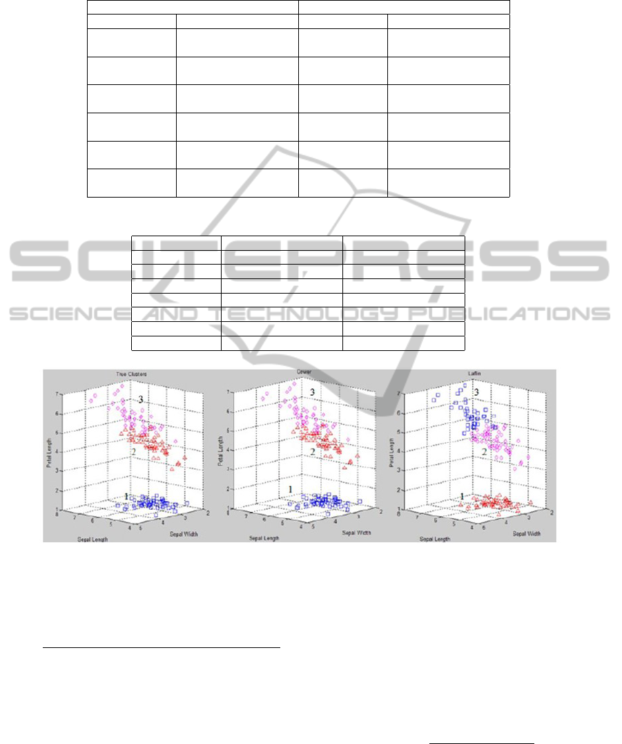
Table 8: F-measure and G-means scores for Mixed datasets. Algorithm: SM (NCut), Splitting points: zero and mean value,
respectively.
F-measure G-means
Dataset GOWER LAFLIN Dataset GOWER LAFLIN
Automobile 0.46 0.44 Automobile 0.49 0.48
0.46 0.46 0.50 0.49
CRX 0.76 0.79 CRX 0.76 0.79
0.76 0.79 0.76 0.79
Dermatology 0.85 0.87 Dermatology 0.86 0.87
0.84 0.82 0.85 0.83
Hepatitis 0.71 0.73 Hepatitis 0.74 0.75
0.73 0.75 0.75 0.77
Post Operative 0.56 0.56 Post Operative 0.57 0.57
0.56 0.56 0.58 0.57
Soybean 0.70 0.70 Soybean 0.72 0.72
0.70 0.70 0.72 0.72
Table 9: F-measure and G-means scores from the NJW (K-means) algorithm (tested on mixed dataset).
F-measure G-means
Dataset GOWER LAFLIN GOWER LAFLIN
Automobile 0.47 0.45 0.48 0.46
CRX 0.76 0.80 0.76 0.80
Dermatology 0.84 0.82 0.86 0.84
Hepatitis 0.71 0.74 0.74 0.76
Post Operative 0.52 0.47 0.53 0.49
Soybean 0.57 0.53 0.61 0.56
Figure 6: Comparison of numeric functions on Iris dataset. (From left) the clusters obtained from the true clusters, the clusters
obtained from the numeric function of the GOWER coefficient, and the clusters obtained from the numeric function of the
LAFLIN coefficient.
Equation 5 can be re-written as:
s(i, j) =
N − (N
1
(1 − s
1
) + N
2
(1 − s
2
) + N
3
(1 − s
3
))
N
(6)
At this point, the GOWER equation given in Equation
3 and the LAFLIN’s coefficient given in Equation 6,
both have similar patterns. They have the same de-
nominator. However, they differ only in the terms in
numerator. As mentioned previously, d
i j
is the dis-
tance or dissimilarity between the two objects i and
j, whereas, (1 − s
1
) is also a dissimilarity measure.
Both functions handle nominal and binary variables
in the same way. Therefore, this implies that the dif-
ference in the equations occurs due to the functions
selected for the numeric attributes which are handled
differently by the two coefficients. This is one of the
reasons that the difference between the performances
of both of the coefficients is very low. In our tests,
we used the Euclidean distance for the LAFLIN’s co-
efficient, whereas, the GOWER coefficient uses the
distance measure given in Equation 7.
d
( f )
i j
=
|x
i f
− x
j f
|
max
h
x
h f
− min
h
x
h f
(7)
We use the two numeric functions with the spec-
tral clustering algorithms and apply them on the Iris
dataset from the UCI repository (Bach and Jordan,
2006) to evaluate their performances. Figure 6 il-
A COMPARATIVE EVALUATION OF PROXIMITY MEASURES FOR SPECTRAL CLUSTERING
39

lustrates the clusters obtained from the true clusters
(left), the clusters obtained from the numeric function
of the GOWER coefficient (middle), and the clusters
obtained from the numeric function of the LAFLIN
coefficient (right). We notice that both of the mea-
sures correctly cluster the objects from true cluster
1. However, the difference between them is clear in
true cluster 2 and cluster 3. Notice that these two true
clusters have objects that overlap near the boundary
of the clusters. The objects located at the boundary
usually have attribute values slightly different from
the other members of their own true clusters. The nu-
meric function for the GOWER coefficient correctly
distinguishes several objects near the boundary. How-
ever, the LAFLIN coefficient, which used the Eu-
clidean distance to compute the distance between the
objects, placed the objects which are located near the
boundary, in two different clusters. We notice that the
clusters formed from this measure have a shape simi-
lar to a sphere. This may be the reason for this mea-
sure performing slightly differently than the function
of the GOWER coefficient.
4.4.1 Discussion
In summary, under certain conditions, the GOWER
similarity coefficient and the LAFLIN coefficient per-
form similarly. The constraints are as follows: 1) the
dataset does not include asymmetric binary variables,
and 2) the distance and similarity measures for each
of the variables are the same. Recall from Section
4.3 that our results for numeric variables indicate that
the Euclidian distance may not be the best choice for
numeric variables. This choice seems to impact the
performance of the LAFLIN coefficient, which may
be improved by using a different distance measure for
the numeric variables.
5 CONCLUSIONS
In cluster analysis, the selection of proximity mea-
sures is a crucial step that has a huge impact on the
quality and usability of the end results. However,
this fact is frequently overlooked, leading to a degrad-
ing of the potential knowledge being discovered. To
address this issue, this paper presents an explorative
and comparative study of the performance of various
proximity measures when applied to the spectral clus-
tering algorithms. In particular, our study address the
question when, and where, the choice of proximity
measure becomes crucial in order to succeed. Our
results indicate that proximity measures needs spe-
cial care in domains where the data is highly imbal-
anced and where in is important to correctly cluster
the boundary objects. These cases are of special inter-
est in application areas such as rare disease diagnosis,
oil spill detection and fraud detection.
Our future work will consider a diverse selection
of datasets. We aim to evaluate if our conclusions
hold for sparse datasets with noise and many missing
values. We will also extend our research to very large
datasets with high dimensionality. For such datasets,
these proximity measures may not perform as per our
expectation. That is, with high dimensions, the data
may become sparse and the distance computed from
these measures may not capture similarities properly.
In such cases, a different set of proximity measures
may be required to deal with the problem of high di-
mensionality.
The selection of the most suitable proximity mea-
sures when specifically aiming to detect outliers and
anomalies is another topic of future research. In order
to reach a conclusion with higher generality, we are
interested to see whether the conclusions drawn from
our paper persist for other clustering algorithms. The
development of additional measures for mixed data
types, especially ones that do not use the Euclidian
distance for numeric data, are also a significant issue
which will benefit from being further researched.
REFERENCES
Abou-Moustafa, K. T. and Ferrie, F. P. (2007). The mini-
mum volume ellipsoid metric. In Proceedings of the
29th DAGM conference on Pattern recognition, pages
335–344, Berlin, Heidelberg. Springer-Verlag.
Aiello, M., Andreozzi, F., Catanzariti, E., Isgro, F., and San-
toro, M. (2007). Fast convergence for spectral cluster-
ing. In ICIAP ’07: Proceedings of the 14th Interna-
tional Conference on Image Analysis and Processing,
pages 641 – 646, Washington, DC, USA. IEEE Com-
puter Society.
Asuncion, A. and Newman, D. (2007). UCI Machine Learn-
ing Repository.
Bach, F. R. and Jordan, M. I. (2003). Learning spectral clus-
tering. In Advances in Neural Information Process-
ing Systems 16: Proceedings of the 2003 conference,
pages 305–312. Citeseer.
Bach, F. R. and Jordan, M. I. (2006). Learning spectral
clustering, with application to speech separation. J.
Mach. Learn. Res., 7:1963–2001.
Boslaugh, S. and Watters, P. A. (2008). Statistics in a nut-
shell. O’Reilly & Associates, Inc., Sebastopol, CA,
USA.
Costa, I. G., de Carvalho, F. A. T., and de Souto, M. C. P.
(2002). Comparative study on proximity indices for
cluster analysis of gene expression time series. Jour-
nal of Intelligent and Fuzzy Systems: Applications in
Engineering and Technology, 13(2-4):133 – 142.
KDIR 2011 - International Conference on Knowledge Discovery and Information Retrieval
40

Everitt, B. S. (1980). Cluster Analysis. Edward Arnold and
Halsted Press, 2nd edition.
Filzmoser, P., Garrett, R., and Reimann, C. (2005). Multi-
variate outlier detection in exploration geochemistry.
Computers and Geosciences, 31(5):579–587.
Fischer, I. and Poland, J. (2004). New methods for spectral
clustering. Technical Report IDSIA-12-04, IDSIA.
Han, J. and Kamber, M. (2006). Data Mining: Concepts
and Techniques, 2nd Ed. Morgan Kaufmann Publish-
ers Inc., San Francisco, CA, USA.
Heinz, G., Peterson, L. J., Johnson, R. W., and Kerk, C. J.
(2003). Exploring relationships in body dimensions.
Journal of Statistics Education, 11(2).
Jain, A. K., Murty, M. N., and Flynn, P. J. (1999). Data
clustering: a review. ACM Computing Surveys,
31(3):264–323.
Japkowicz, N. and Shah, M. (2011). Performance Evalua-
tion for Classification A Machine Learning and Data
Mining Perspective (in progress): Chapter 6: Statisti-
cal Significance Testing.
Kaufman, L. and Rousseeuw, P. (2005). Finding Groups
in Data: An Introduction to Cluster Analysis. Wiley-
Interscience.
Kubat, M., Holte, R. C., and Matwin, S. (1998). Machine
learning for the detection of oil spills in satellite radar
images. Machine Learning, 30(2 - 3):195 – 215.
Larose, D. T. (2004). Discovering Knowledge in Data: An
Introduction to Data Mining. Wiley-Interscience.
Lee, S. and Verri, A. (2002). Pattern Recognition With Sup-
port Vector Machines: First International Workshop,
Svm 2002, Niagara Falls, Canada, August 10, 2002:
Proceedings. Springer.
Luxburg, U. (2007). A tutorial on spectral clustering. Statis-
tics and Computing, 17(4):395–416.
Meila, M. and Shi, J. (2001). A random walks view of spec-
tral segmentation. In International Conference on Ar-
tificial Intelligence and Statistics (AISTAT), pages 8–
11.
Ng, A. Y., Jordan, M. I., and Weiss, Y. (2001). On spectral
clustering: Analysis and an algorithm. In T. G. Diet-
terich, S. B. and Ghahramani, Z., editors, Advances in
Neural Information Processing Systems, volume 14,
pages 849–856.
Paccanaro, A., Casbon, J. A., and Saqi, M. A. (2006). Spec-
tral clustering of protein sequences. Nucleic Acids
Res, 34(5):1571–1580.
Shi, J. and Malik, J. (2000). Normalized cuts and image
segmentation. IEEE Transactions on Pattern Analysis
and Machine Intelligence, 22(8):888–905.
Steinbach, M., Karypis, G., and Kumar, V. (2000). A
comparison of document clustering techniques. KDD
Workshop on Text Mining.
Teknomo, K. (2007). Similarity Measurement. Website.
Verma, D. and Meila, M. (2001). A comparison of spectral
clustering algorithms.
Webb, A. R. (2002). Statistical Pattern Recognition, 2nd
Edition. John Wiley & Sons.
Witten, I. H. and Frank, E. (2005). Data Mining: Practi-
cal Machine Learning Tools and Techniques. Morgan
Kaufmann, 2 edition.
A COMPARATIVE EVALUATION OF PROXIMITY MEASURES FOR SPECTRAL CLUSTERING
41
