
MOBILE ROBOT
A Complete Framework for 2D-path Planning and Motion Planning
Giuseppe Zuffanti
1,2
and Costantino Scozzafava
3
1
Lagrange Project-CRT Foundation, Institute for Scientific Interchange Foundation, 10133 Turin, Italy
2
Department of Computer Science, University of Turin, Turin, Italy
3
Erxa S.r.l., 10149 Turin, Italy
Keywords:
Path planning, Motion planning, Roadmap graph, Potential field, Look-ahead, Obstacle avoidance, Attraction
point, Dynamic environment.
Abstract:
In this work we focus on the problem of 2D path planning and motion planning for a mobile robot. The
goodness of a path planning and motion planning methods can be evaluated primarily through the parameters
such as safety of generated trajectory speeds and robustness against dynamic changes of the environment. In
all applications that use mobile robots, the motion planning problem is of crucial importance. According to
different applications one can put emphasis on the previous characteristics listed, potentially to the detriment
of the others. Typically, methods that generate high trajectory speeds for the navigating robot appears to be
less robust and safe. The importance that the path planning and the motion planning problem play in practical
applications is also demonstrated by the several techniques developed to tackle them. We propose a complete
framework which creates a clear shortest path for a robot in an environment with static obstacles and generates,
in real time, the accurate trajectory taking into account the presence of dynamics obstacles. Application of the
framework to the case of a differential drive robot in a dynamic indoor environment is shown and the proposed
approach has been tested both with simulation and real data.
1 INTRODUCTION
One of the main tasks of a wheeled mobile robot
(WMR) is the capability of plan and execute collision-
free paths when moving around (Budanov and De-
vyanin, 2003). While the problem of path planning
has been historically addressed as a purely geometric
issue (since the piano-mover problem), in the case of
a real robot moving in its surroundings several new
constraints have to be considered and added to the
original problem position (Canny, 1988), (Latombe,
1991), (LaValle, 2006). Typical such constraints arise
when taking into account the anholonomy of the robot
kinematics model, dynamic changes in the surround-
ings and uncertainties related to the sensors measure-
ments (Siciliano et al., 2008). In this work we de-
scribe a framework for the solution of the path plan-
ning of a WMR in which the main problem is di-
vided in two sub-problems: 1) planning of a geomet-
ric, collision-free, motion and 2) execution of the mo-
tion in a dynamic scenario. Finally further dynamical
constraints on the generated trajectories are imposed
to let the motions be generated at the maximum allo-
wed speed taking into account the safety of both the
robot it-self and the surrounding objects (LaValle and
Kuffner, 1999).
The proposed solution has been implemented and
tested using a robotic platform Pioneer P3DX and
a proprietary real-time control software system (RT-
Platform).
2 PATH PLANNING FOR
DYNAMIC ENVIRONMENT
Nevertheless, in most cases, moving directly to the
goal isn’t possible due primarily to the structure of the
surroundings. Besides, also if the problem of deter-
mining a feasible way to the goal is solved, one must
take into account that unexpected dynamic obstacles
can cross the robot trajectory. In an indoor scenario
these problems can be directly related to moving to
some room in an office (or a house) and avoiding col-
lisions with persons and with not previously known
objects (chairs, moving people, etc.). Such a kind of
417
Zuffanti G. and Scozzafava C..
MOBILE ROBOT - A Complete Framework for 2D-path Planning and Motion Planning.
DOI: 10.5220/0003648504170426
In Proceedings of the 8th International Conference on Informatics in Control, Automation and Robotics (MORAS-2011), pages 417-426
ISBN: 978-989-8425-75-1
Copyright
c
2011 SCITEPRESS (Science and Technology Publications, Lda.)

scenario (non-structured, partially dynamic) will be,
for the rest of the document, the reference scenario in
which hypotheses and experiments have their validity.
Accordingly to the problem decomposition we
identified two main functional modules able to cope
with the given sub-problems. They are the Path Plan-
ner OFF-Line Module and the Path Planner ON-Line
Module.
2.1 Path Planner OFF-line Module
An important influence on the quality of the path
founded by the Path Planner OFF-Line Module, is the
quality of the graph that represents the free space. For
to represent the free space and for to build the cor-
responding graph we have studied the map building
techniques present in literature (Veeck and Burgard,
2004), (Masehian and Movafaghpour, 2009). All of
them use the information from the on-board sensors
of the robot. In the map building process it’s possible
to identify two main phases:
1. acquiring information through sensors about the
characteristics of environment and objects sur-
rounding the robot;
2. processing this information to obtain a summary
of the space around the robot, discarding the in-
consistent information due to the uncertainty and
imprecision of sensors.
There are many possible solutions to accomplish
these two steps and to get maps, but those the most
often and successfully used are based on grid maps,
on topological maps or on geometrical maps.
We developed a specific Geometric Map Build-
ing algorithm (GMB) capable of building, in a dy-
namically and incrementally approach, a geometric
map of the environment using sonar range or laser
scanner. The global map is composed of two main
type of contours, the first set of contours represents
the whole free space while the second set represents
the entire holes contours. We preferred the geomet-
ric map representation because we have a low mem-
ory occupancy, especially in situations where is very
broad. This choice is also useful because is better
to adapt representation of the points constituting the
map if necessary corrections due to errors caused by
the detection system of the robot, through its analyt-
ical operations of vector geometry. Starting from a
result of the dedicated map building module which
represents the 2D environment, a first goal was to ap-
ply a mesh algorithm to obtain a triangulation of free-
space.
Specifically, a standard 2D mesh geometry rep-
resentation is used for depicting an hypothetical en-
vironment map using as input the result of the map
building module. This is the potentially viable areas
by the robot. In general the term mesh refers to a set
of polygons such that two of its elements do not inter-
sect, or share a vertex, or an edge. Each polygon ap-
proximates a portion of the surface. Meshes are easy
to represent, to manipulate, to display and are also re-
constructed from irregularly sampled data. In particu-
lar we have chosen the triangular mesh, for which in-
ternal representation we stored geometric information
such as the position of the vertices of triangles, the
connectivity and the relationships between triangles
themselves. The used mesh algorithm can produce a
Constrained Delaunay Triangulation (CDT) (Delau-
nay, 1934): a construction of grids with finite trian-
gular element on plans domain filling generic forms.
The triangulation mesh algorithm is an exact decom-
position method of the free-space that produce a col-
lection of non-overlapping cells (triangles) and the
union of these, exactly equals the free-space or rather
the space in R2 where the robot can move without
colliding by static obstacles.
To get a free-path to move the robot from a start to
a goal is to keep it moving only over triangles that rep-
resent the free-space, or the part of the environment
completely devoid of obstacles (Lien et al., 2003). It
was thought to obtain a free-path as follows:
1. generate a basic Roadmap, always available in the
data structure, representing the undirected graph
G = (V , E ) where V is the set of all centroids of
the triangles forming the mesh in the free-space,
E is the set of all edges that connect each node V
with all adjacent nodes (minimum one and maxi-
mum three adjacent nodes for each triangle)
2. starting from a roadmap graph, a start point and
a goal point belonging to the free-space, on the
roadmap graph it is built, with Dijkstra algorithm,
a MST(Minimum Spanning Tree) or minimum
weight spanning tree. The graph is weighted by
the length of each edges of the graph. The MST
has as its root the centroid of the triangle closer to
the start point of the robot position.
3. if we denote by C
s
the centroid of the triangle in
the free-space closer to the start point and with C
g
the centroid of the triangle in the free-space closer
to the point of goals, we may define the Shortest-
Path (SP) as the path in the roadmap graph joining
C
s
and C
g
plus two edges, one that connects the
start with C
s
and one that connects C
g
with the
goal. This path represent a safety shortest path in a
free space that the Path Planner ON-Line Module
will use to planned a safe and smooth trajectory.
To ensure the MST covers the free-space really navi-
gable by the robot, a further prune operation is made
ICINCO 2011 - 8th International Conference on Informatics in Control, Automation and Robotics
418
in the MST building phase to leave out the nodes of
the graph that represents all the centroids of a trian-
gles mesh where the robot can not enter because of
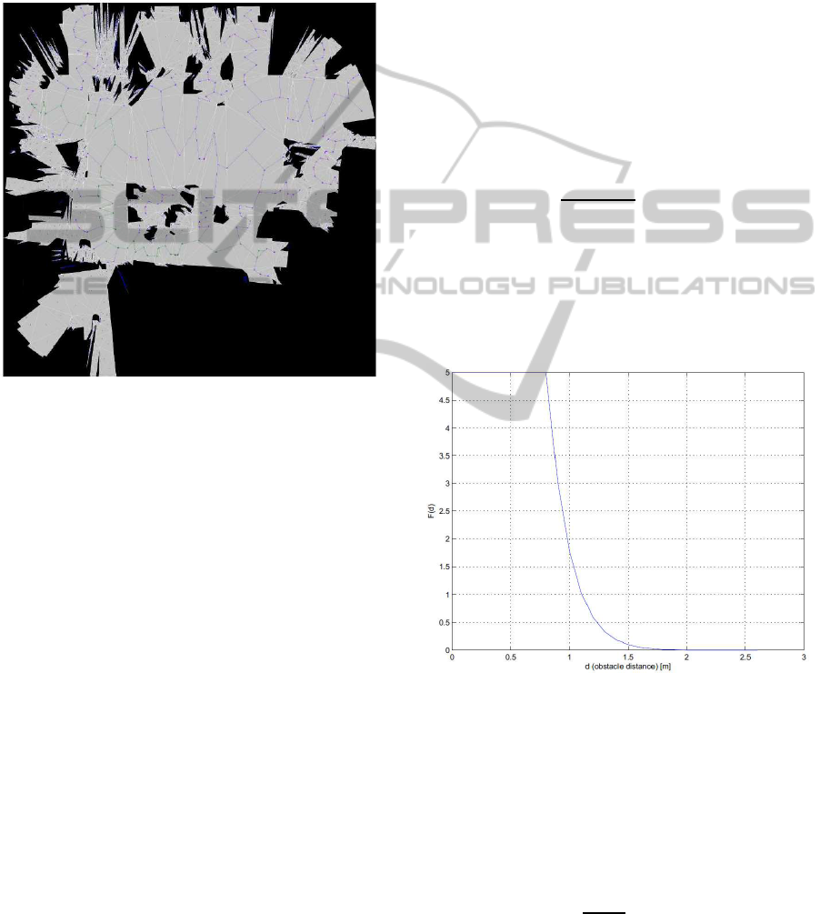
their size. Fig.1 illustrates an example of a Pruned
Minimum Spanning Tree (PMST) built on a roadmap
graph which covers a large portion of the free space
in a real indoor environment.
Figure 1: In the bottom left area of the picture one can ob-
serve the result of the graph-edges pruning (corridor is nar-
rower than the size of the robot).
2.2 Path Planner ON-Line Module
The Path Planner OFF-Line Module allows to obtain
a set-point, or rather the list of the triangles centroids
provided by shortest-path algorithm, which are useful
as reference for the robot to move in safe areas, free
of static obstacles. The Path Planner ON-Line is the
module phase that implement all those algorithms ca-
pable of managing the proper handling of the robot
and the obstacle avoidance in case of mobile or un-
expected obstacles. This is the stage where it should
consider the dynamic characteristics of a real envi-
ronment (moving obstacles, local changes of the map
built during off-line phase, etc...), and then the reason-
ing capabilities and the reactive abilities of the mobile
robot. To manage the robot movements an interpola-
tion strategy between the current robot position and
the goal position has been tested, to generate trajecto-
ries keeping the mobile robot’s kinematic constraints.
We have chosen to exploit the concept of Attraction
Points (Geraerts and Overmars, 2007), a very typical
approach in the potential field methods, as follows:
the robot is attracted by an appropriate node of SP at
a time, and when this target is no longer valid an op-
portune target node is activated. Once all centroids of
the SP have been activated the robot it is performed a
last move toward the point of ultimate goal.
The problem of obstacle avoidance has been faced
using the potential field method. The function that de-
scribes this field is generally the sum of distinct com-
ponents depending on attractive and repulsive forces
(Rimon and Koditschek, 1992). The global motions
of the robot is mainly guided by a dynamically attrac-
tion point that represent the principal oracle to follow
to find the safe way to identify the best way to goal.
The attraction point attracts the robot with force F
a
.
Let x be the current robot position, p(x) be the op-
portune node position of PP, d be the Euclidean dis-
tance between x and p(x), b be the sensor beam.
The F
a
is defined as:
F
a
=
(x− p(x))
d
· min(d, b). (1)
A repulsive force F
r
is generated by dynamic local
obstacles or rather the obstacles in the environment
around to the robot that there did not exist or were far
when the SP is created. A repulsive force deflection
F
d
determines the behaviour that the robot must take
each obstacle is detected (Fig.2).
Figure 2: Repulsive force deflection.
Let d
i
be the Euclidean distance between robot po-
sition x and o
i
(a point corresponding to a sensor ob-
stacle measure), s be the size robot, F
R
sat
be the repul-
sive force saturation, D
Z
i
be the Euclidean distance
between x and o
i
to reset F
d
, n be the shape of F
d
.
The F(d
i
) is defined as:
F(d
i
) =
F
R
sat
if d
i
< s
F
R
sat
·
d
i
−D
Z
i
s−D
Z
i
n
if s ≤ d
i
≤ D
Z
i
0 if d
i
> D
Z
i
(2)
MOBILE ROBOT - A Complete Framework for 2D-path Planning and Motion Planning
419
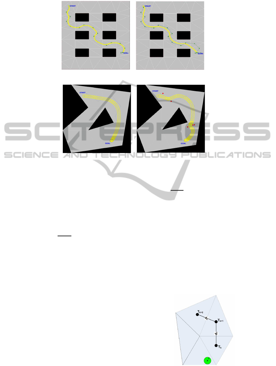
(a) Safe trajectory (Not optimized). (b) Safe and optimized trajectory by
lookahead.
(c) Trajectory without dynamics obsta-
cles.
(d) Modified trajectory caused by unex-
pected local dynamics obstacles.
Figure 3: Examples of different trajectory in a simulate world.
Let m be the number of surround obstacles measured
by o
i
, y
i
be the position of surround obstacles at o
i
distance, d
i
be the Euclidean distance between robot
position x and o
i
.
The F
r
is defined as follows:
F
r
= −
m
∑
i=1
y
i
− x
d
i
· F(d
i
). (3)
The final force F is calculated as:
F = F
a
+ F
r
. (4)
By calculating the final force F we can get the op-
portune sub-target in the free-space that the Motion
Planning module may use to calculate the trajectory
of the robot respecting kinematic constraints (Chitsaz
et al., 2006). Additional strategies to smooth trajec-
tories have been studied and implemented to reduce
redundant paths and robot acceleration/deceleration
phases. This was possible introducing an appropri-
ate look-ahead feature (Fig.4) allowing the Path Plan-
ner ON-Line Module to use as main attraction point
a proportionally point onto the edge between the next
two centroids of the SP.
The new target is calculated as follows:
LookAheadON ← near(P
r
, T
c
)
if LookAheadON = true then
T
c
← α
d
1
d
1
+d
2
(T
k+2
− T
k+1
)
else
T
c
← T
k
end if
where,
P
r
= robot pose,
T
c
= current target,
T
k
= centroid of k-th triangle,
T
k+1
= centroid of (k+1)-th triangle,
T
k+2
= centroid of (k+2)-th triangle,
α = percentage parameter,
d
1
= Euclidean distance between T
k+1
and T
k
,
d
2
= Euclidean distance between T
k+2
and
T
k+1
,
Figure 4: Example of look-ahead technique.
ICINCO 2011 - 8th International Conference on Informatics in Control, Automation and Robotics
420
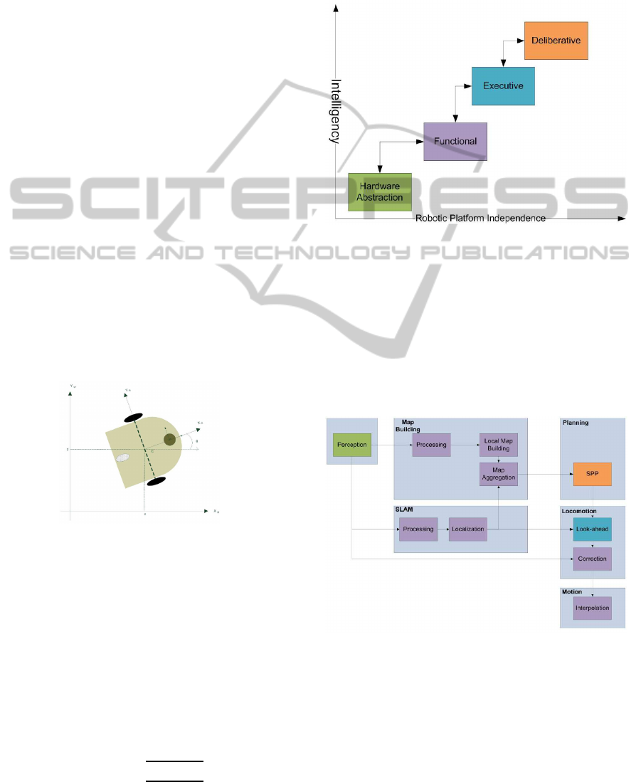
Fig.3(a), Fig.3(b) illustrates two different types of
trajectory of the robot obtained with different tech-
nique in a simulate world (box size:40x40 [m]). The
first simulative results showed that the robot, in a cer-
tain narrow area of the map, could not divert its tra-
jectory in time because of speed. To work around
the problem we introduced a feed-rate control speed
that proportionally modify the speed parameter of
the robot in function of nearest obstacles surround in
agreement with the max speed parameter and max ac-
celeration parameter of the robot. An opportune value
saturation is applied to prevent instable and unsafe sit-
uations. Fig.3(c), Fig.3(d) illustrates an example of
the reactivity of the Path Planner ON-Line Module
(box size:10x10 [m]).
3 THE ROBOT AND ITS
SOFTWARE CONTROL
ARCHITECTURE
In order to test the proposed solution a real-time soft-
ware platform (RT-Platform) has been designed and
developed to control a mobile robot (Pioneer P3DX).
The robot has been equipped with an external laser
range scanner (Sick LMS 100) and a Acer-One net-
book executing the control software algorithms on a
XP tailored OS.
Figure 5: Robot kinematic model.
The robot kinematic model (Fig. 5) used for mo-
tion interpolation is based on the simpler model given
by the following equation:
˙x(t)
˙y(t)
˙
θ(t)
=
υ(t)cos(θ(t))
υ(t)sin(θ(t))
ω(t)
(5)
where υ(t) and ω(t) represent, respectively, the linear
and angular velocities of the robot body fixed frame
defined as:
υ(t)
ω(t)
=
"
R
ω
R
(t)+ω
L
(t)
2
R
ω
R
(t)−ω
L
(t)
D
#
(6)
where,
ω
R
(t) = angular speed of the right wheel,
ω
L
(t) = angular speed of the left wheel,
R = wheel radius (before calibration),
D = wheel centers distance.
Figure 6: Functional, abstract layers of the proposed archi-
tecture.
Our proposed architecture is based on (Alami et al.,
1998). It can be decomposed in four layers: a delib-
erative level, an executive level, a functional level and
an hardware abstraction (Fig.6).
In the previous layered scheme the data flowing
through path planning modules is summarized in
Fig.7.
Figure 7: Data flows and transformations along the path
planning ’toolchain’. The color of each block refers to the
architectural functional layer it belongs.
3.1 Data Perception
The Perception module collects the laser raw data at
a frequency of 2Hz and stores them in a real-time
database. It then signals to all interested modules that
MOBILE ROBOT - A Complete Framework for 2D-path Planning and Motion Planning
421

fresh data are ready in the database. A timestamp
is coupled to every newly acquired set of data. The
mobile robot P3DX (Fig.8) has been equipped with
a SICK LMS-100 Laser Scanner mounted on the top
of the robot. The LMS-100 laser scanner has been
configured to collect range measurement over a 270
◦
range, with 0.25
◦
of angular resolution. Moreover the
scanning plane of the LMS-100 has been positioned at
an elevation, from the floor, of around 35cm. Due to
the short range measured in an indoor environment, at
this stage of the work, no calibration of the sensor ori-
entation with respect the parallelism to the floor was
made; while the mounting offset with respect of the
body-fixed frame F
r
of the robot was estimated to be
at around [0.20] meters (Fig.5).
Finally we integrated a software driver for the sen-
sor in the RT-Platform architecture through a USB-to-
serial connection. The software driver provides raw
data measured by the sensor to all subscribed soft-
ware components leaving the choice of how to pro-
cess them to each component.
Figure 8: Pioneer P3DX.
3.2 Data Processing
SLAM Function. The raw data stored in real-time
database are processed in order to extract corner and
line features eligible to become new or yet known
landmarks to be entered in the Update phase of the
SLAM algorithm.
Map Building Function. The raw data stored in real-
time database are processed in order to build a local
map of the surroundings.
3.3 Local Map Aggregation and
Planning
After a Local Map has been built it’s fused in a Global
Map. The fusion, or aggregation, operation is per-
formed taking into account the estimated robot posi-
tion (SLAM) and the yet existing landmarks. Once
the Global Map has been updated it’s possible for the
Path Planning OFF-Line Module to deliberate a suit-
able path to a goal position. The path is the input for
the Locomotion Module.
3.4 Locomotion
The path generated by the Path Planner OFF-Line
Module is the input for the Locomotion Module (Al-
bagul and Wahyudi, 2004). It will provides two main
functionalities:
1. trajectory smoothing via a spatial look-ahead;
(Liang and Liu, 2004)
2. dynamic obstacle detection.
Look-ahead. The look-ahead sub-function, ac-
cordingly to dynamic obstacle detection, is able
to shorten and smooth the route to the final goal
by foreseeing which targets of the original path
have to be reached and at which instant in time the
current target can be replaced by its successor (Fig.9).
Figure 9: The green circles, representing the intermediate
targets ofa path, are used to smooth the generated trajectory.
Obstacle Detection. Detecting dynamic obstacle
while moving along a path is a fundamental function
both for robot safety and goal effective reachability.
The laser raw data are processed in order to measure
the reachability of the current and next targets. The
information is 1) propagated to the look-ahead func-
tion and 2) used to correct the robot speeds in order to
have always enough space for to brake.
3.5 Motion Interpolation
The Motion Interpolation module has in charge the
goal of to generate speed targets for the Pioneer P3DX
robotics platform at a frequency of 10 Hz. Given
the kinematics model in equation 5, it has been re-
visited providing a special choice for the system state
equations as shown in (Aicardi et al., 1994). Then a
state-dependent, smooth, non-linear control law gen-
erating the command vector [υ, ω]
T
has been proven
to drive the robot in the desired final position and ori-
entation. The closed loop chain generating the speed
commands for the robot is shown in Fig.10.
ICINCO 2011 - 8th International Conference on Informatics in Control, Automation and Robotics
422
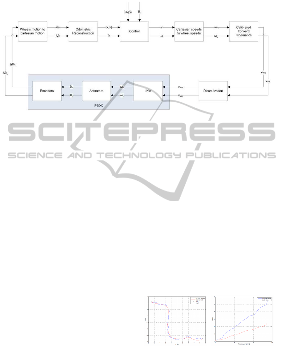
Figure 10: Closed loop control schema.
4 RESULTS
The simulative and experimental results show the ef-
fectiveness of the approach. The Locomotion module
has been made robust in case of replanning because
the high level system autonomously reconfigures it-
self to correctly achieve the mission. The implemen-
tation of the all module in a variety of dynamic indoor
environment shows the efficiency of the approach as
a good navigation framework for a mobile robot.
The simulative and experimental results have
shown the effectiveness of the proposed approach.
Firstly, experimental test-cases have been built in or-
der to test the behavior of every specific module (Path
Planner OFF-Line Module only, Path Planner ON-
Line Module only); then the complete planning and
control chain has been closed in order to let the robot
(Pioneer P3DX Fig.8) plan and navigate in an un-
structured indoor scenario. In Fig.11(a) are shown
both the real trajectory of the robot under the in-
fluence of modifications induced by the look-ahead
strategies and the decrease of trajectory duration in
time (Fig.11(b)) due to the elimination of intermedi-
ate targets.
To verify the look-ahead improvements of the
generated trajectories we performed 50 runnings of
the robot over 5 different path sets; all paths were
generated inside the Erxa s.r.l. office letting the robot
moves from one room to another. Moreover between
paths of the same set were slight differences due to the
variable presence of chairs or baskets. For each set of
paths the average time and length of the trajectories
execution has been evaluated. The results are shown
in Table1, where, for each column, one can observe
the average lengths and average times with and with-
out the Look-ahead functionality working. For each
paths set an increase of performances for both length
and time has been evaluated as the percent ratio of the
cases without Look-ahead over the cases with Look-
ahead. The same trajectory has then been executed
by introducing, along the robot motion, a number of
dynamic obstacles as shown in Fig.12(c) (red dots)
to demonstrate the capability of obstacle avoidance
via the local trajectory deformation; the obstacles, de-
tected at run-time, are used to smoothly modify the
local targets to the robot.
The resulting behavior allowed the robot to au-
tonomously move in a scenario where people was
moving around. Furthermore, in order to improve
the safety of the people and of the robot it-self, a
proximity detection alert functionality based on sonar
range readings has been implemented to eliminate the
risk of collision against high-speed moving objects; in
fact in this cases the relatively low frequency of laser
range readings update could result in unseeing some
quickly moving obstacle.
(a) The comparison of two trajecto-
ries with and without look-ahead.
(b) The performance of look-ahead.
Figure 11: Results of different trajectory in a static real
world.
MOBILE ROBOT - A Complete Framework for 2D-path Planning and Motion Planning
423
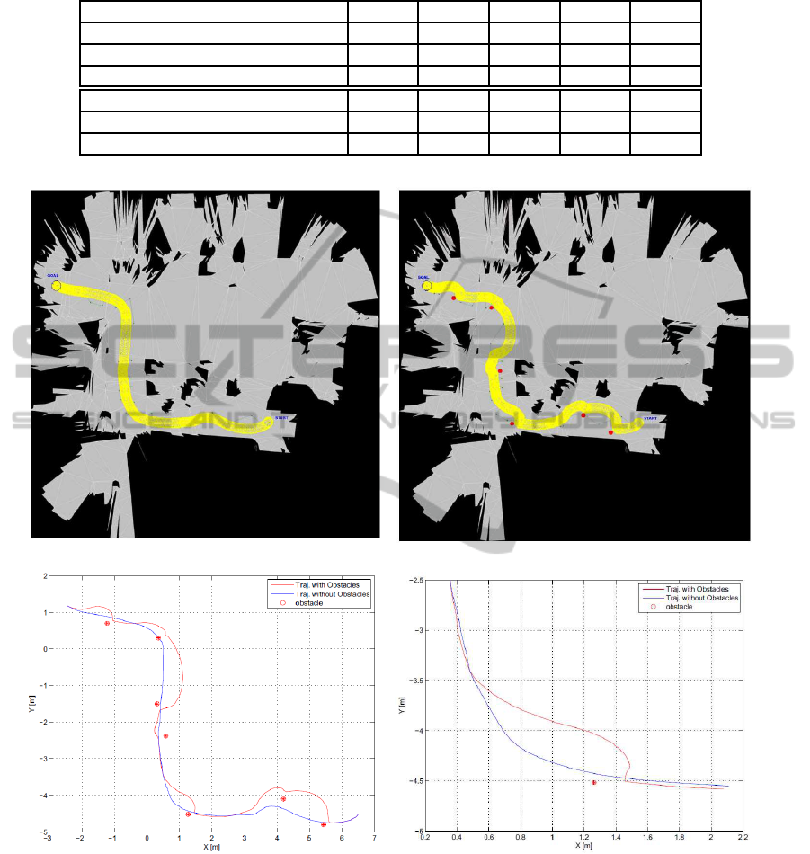
Table 1: A comparison between trajectory lengths and execution times with and without look-ahead functionality active on
the Pioneer P3DX moving in Erxa office. The percentages are the ratios between the obtained results in two cases.
Path1 Path2 Path3 Path4 Path5
Traj.Lenght With Look-Ahead [m] 13.975 21.223 19.214 28.347 24.231
Traj.Lenght Standard [m] 15.129 23.214 20.146 32.421 27.215
Performance[%] 7.63 8.58 4.63 12.57 10.96
Traj.Time With Look-Ahead [s] 12.536 18.949 17.216 23.622 21.405
Traj.Time Standard [s] 30.128 45.517 38.742 62.953 51.349
Performance[%] 58.39 58.37 55.56 62.48 58.31
(a) A true trajectory in a real static environment. (b) The newtrajectory caused by unexpected local dynamics obstacles.
(c) The comparison of two trajectories. (d) Zoom trajectory close an obstacle.
Figure 12: Results of different trajectory in a static and dynamic real indoor environment.
5 CONCLUSIONS
In this work we have shown how the path planning
problem for a wheeled mobile robot can be decou-
pled in two sub-problems: a problem related to the
geometric, collision-free, path search and a problem
related to the path execution in a dynamic world. Both
the solutions rely on the use of laser sensors; the first
for building a static map of the surroundings, while
the second for avoiding dynamic changes of the sur-
roundings it-self. Then the validity of the solution has
been demonstrated by its implementation in a soft-
ICINCO 2011 - 8th International Conference on Informatics in Control, Automation and Robotics
424
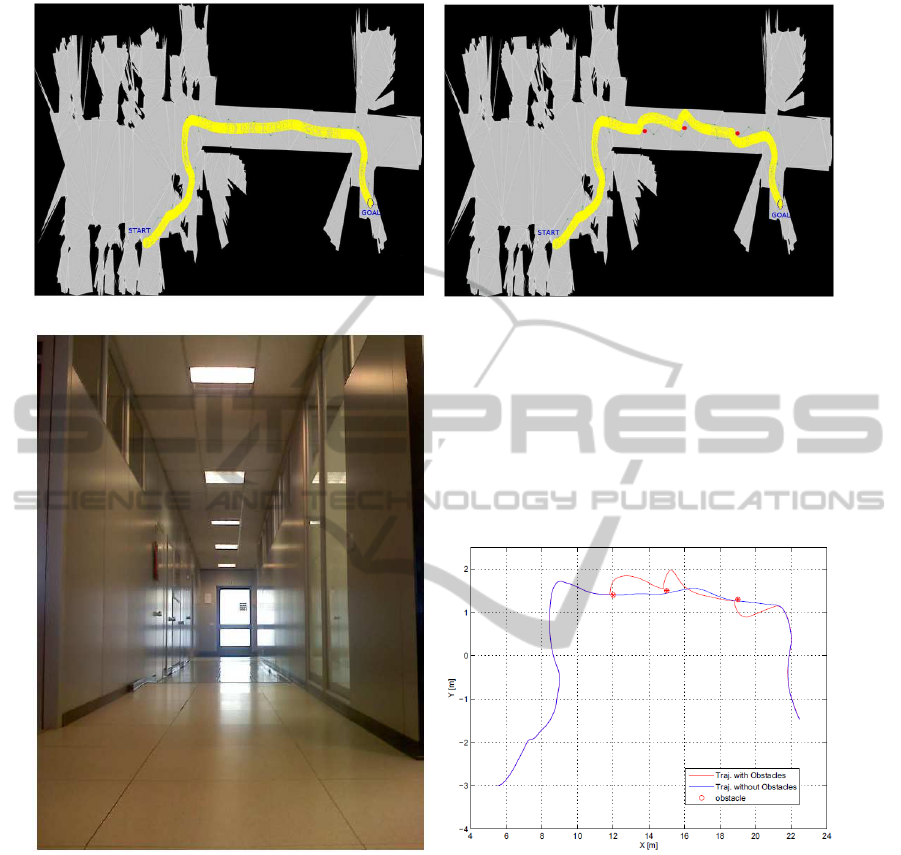
(a) A true trajectory in another real static environment. (b) The newtrajectory caused by unexpected local dynamics obstacles.
(c) The corridor of the office. (d) The comparison of two trajectories.
Figure 13: Results of different trajectory in another static and dynamic real indoor environment.
ware control architecture for a wheeled mobile robot.
Because the collision-free path generation is based on
a self-built map that is constantly updated by new per-
ceived measures, no pre-configured maps of the sur-
roundings are needed.
Finally the functional and operational decoupling
of the solutions gives the possibility to study, de-
velop and test different strategies for each of the sub-
problems. Furthermore we deployed other algorithms
that are not present on this work that allowed to cou-
ple our PP module and MP module with a control
loop involving simultaneous localization and map-
ping. The performed experimentations within a real
dynamic environment of these extensions have given
good result in terms of safety, speed, path shortness,
smooth trajectory and reactivity.
Interesting topics for future researches and future
goals are a 1) closer integration of path planning mod-
ules with SLAM and Navigation functions, and 2) de-
veloping a software framework for fully autonomous
exploration and navigation of unstructured worlds.
MOBILE ROBOT - A Complete Framework for 2D-path Planning and Motion Planning
425

ACKNOWLEDGEMENTS
This research has been funded by the Lagrange
Project (fostered and supported by CRT Foundation
and ISI Foundation) and the Erxa S.r.l.. The scientific
supervision is partly of the Department of Computer
Science, University of Turin.
REFERENCES
Aicardi, M., Casalino, G., Balestrino, A., and Bicchi, A.
(1994). Closed loop smooth steering of unicycle-like
vehicles. In Decision and Control, 1994., Proceed-
ings of the 33rd IEEE Conference on, volume 3, pages
2455 –2458.
Alami, R., Chatila, R., Fleury, S., Ghallab, M., and Ingrand,
F. (1998). An architecture for autonomy. International
Journal of Robotics Research, 17:315–337.
Albagul, A. and Wahyudi (2004). Dynamic modeling and
adaptive traction control for mobile robots. In Indus-
trial Electronics Society, 2004. IECON 2004. 30th An-
nual Conference of IEEE, volume 1, pages 614 – 620.
Budanov, V. M. and Devyanin, Y. A. (2003). The motion of
wheeled robots. Journal of Applied Mathematics and
Mechanics, 67(2):215 – 225.
Canny, J. F. (1988). The Complexity of Robot Motion Plan-
ning. MIT Press, Cambridge, MA.
Chitsaz, H., LaValle, S. M., Balkcom, D. J., and Mason,
M. T. (2006). Minimum wheel-rotation paths for
differential-drive mobile robots. In Proceedings IEEE
International Conference on Robotics and Automa-
tion.
Delaunay, B. N. (1934). Sur la sphre vide. Bulletin of
Academy of Sciences of the USSR, 6:793800.
Geraerts, R. and Overmars, M. H. (2007). The corridor map
method: Realtime high-quality path-planning. In Pro-
ceeding IEEE International Conference on Robotics
and Automation, page 10231028.
Latombe, J. C. (1991). Robot Motion Planning. Kluwer,
Boston, MA.
LaValle, S. M. (2006). Planning Algorithms. Cambridge
University Press, Cambridge, UK, 1st edition.
LaValle, S. M. and Kuffner, J. J. (1999). Randomized kino-
dynamic planning. In Proceedings IEEE International
Conference on Robotics and Automation, page 73479.
Liang, T. C. and Liu, J.-S. (2004). A bounded-curvature
shortest path generation method for car-like mobile
robot using cubic spiral. In Proceedings IEEE/RSJ
In- ternational Conference on Intelligent Robots and
Sys- tems, page 28192824.
Lien, J.-M., Thomas, S. L., and Amato, N. M. (2003). A
general framework for sampling on the medial axis
of the free space. In Proceedings IEEE Interna-
tional Conference on Robotics and Automation, page
44394444.
Masehian, E. and Movafaghpour, M. A. (2009). An adap-
tive sequential clustering algorithm for generating
poly-line maps from range data scan in mobile robot
explorationby. In International Conference on Au-
tomation Technology.
Rimon, E. and Koditschek, D. E. (1992). Exact Robot Nav-
igation Using Artificial Potential Fields. IEEE Trans.
Robot. & Autom., 8(5):501–518.
Siciliano, B., Sciavicco, L., Villani, L., and Oriolo, G.
(2008). Robotics: Modelling, Planning and Control.
Springer Publishing Company, Incorporated.
Veeck, M. and Burgard, W. (2004). Learning polyline maps
from range scan data acquired with mobile robots.
In International Conference on Intelligent Robots and
Systems.
ICINCO 2011 - 8th International Conference on Informatics in Control, Automation and Robotics
426
